Milvus Community Conf 2020_Facebook AI Research:An Introduction to Faiss

1 .An introduction to Faiss and similarity search Matthijs Douze, Jeff Johnson Facebook AI Research 

2 .Work context 

3 . Facebook AI Research “Advancing the state-of-the- art in artificial intelligence through open research for • Part of the larger AI Group at Facebook the benefit of all.” • More research focused computer machine vision learning grounding LONDON Facebook interaction & PAR IS Natural S E AT TL E AI communication MON TR E AL language NEW YOR K research MENLO PA RK PIT TSB URGH understaning TEL AVIV reinforcement speech learning processing 

4 . About us • Matthijs Douze • Jeff Johnson • Based in Paris (France) • Based in Los Angeles (USA) • at Facebook since end 2015 • At Facebook since 2013 • similarity search • novel GPU and FPGA/ASIC • embeddings algorithms for machine learning • unsupervised learning • the author of most of the original PyTorch GPU backend • 10 years at INRIA (research institution) • image/video indexing • BSE in Computer Science from • large-scale 3D reconstruction Princeton University 

5 .Embeddings 

6 .Content embeddings Text embedding (word2vec, Post embedding fastText) Face embedding Video embedding typical: d=100-1000 (dense) User embedding Image Relationship Embedding embedding (CNN layer) 

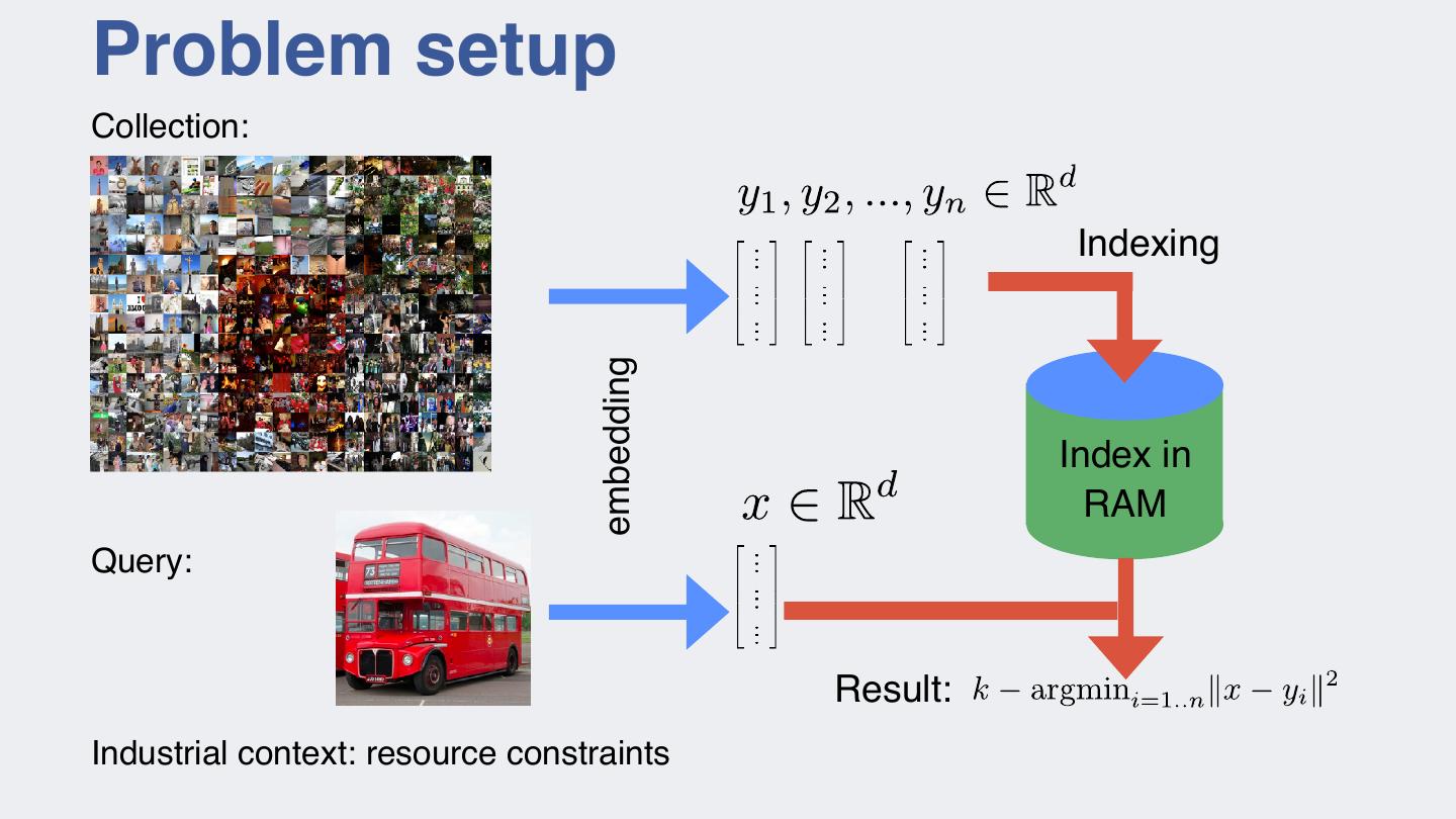
7 .Problem setup Collection: Indexing embedding Index in RAM Query: Result: Industrial context: resource constraints 

8 .Problem setup - classification Training: d w1 , w2 , ..., wn 2 R large set of linear classifiers Indexing on embeddings embedding Index in RAM Object to classify: MIPS Result: k argmaxi=1..n hx, wi i k argmaxi=1..n < x, yi > typical use: recommendation 

9 .Faiss 

10 .The Faiss library • C++ library • Transparent: everything is exposed — no private fields, few abstractions • Few dependencies (only BLAS) • Basic object: the index • in RAM • Train / add / search • Layers above: • Python wrapper • Distributed implementation • database primitives (remove / load-store / filter on other criteria) 

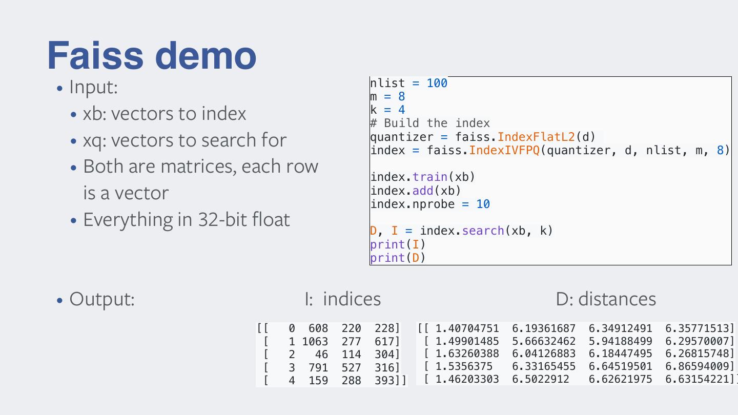
11 .Faiss demo nlist = 100 • Input: m = 8 • xb: vectors to index k = 4 # Build the index • xq: vectors to search for quantizer = faiss.IndexFlatL2(d) index = faiss.IndexIVFPQ(quantizer, d, nlist, m, 8) • Both are matrices, each row index.train(xb) is a vector index.add(xb) index.nprobe = 10 • Everything in 32-bit float D, I = index.search(xb, k) print(I) print(D) • Output: I: indices D: distances [[ 0 608 220 228] [[ 1.40704751 6.19361687 6.34912491 6.35771513] [ 1 1063 277 617] [ 1.49901485 5.66632462 5.94188499 6.29570007] [ 2 46 114 304] [ 1.63260388 6.04126883 6.18447495 6.26815748] [ 3 791 527 316] [ 1.5356375 6.33165455 6.64519501 6.86594009] [ 4 159 288 393]] [ 1.46203303 6.5022912 6.62621975 6.63154221]] 

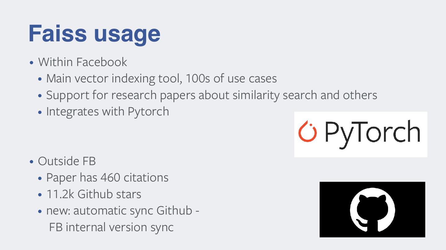
12 .Faiss usage • Within Facebook • Main vector indexing tool, 100s of use cases • Support for research papers about similarity search and others • Integrates with Pytorch • Outside FB • Paper has 460 citations • 11.2k Github stars • new: automatic sync Github - FB internal version sync 

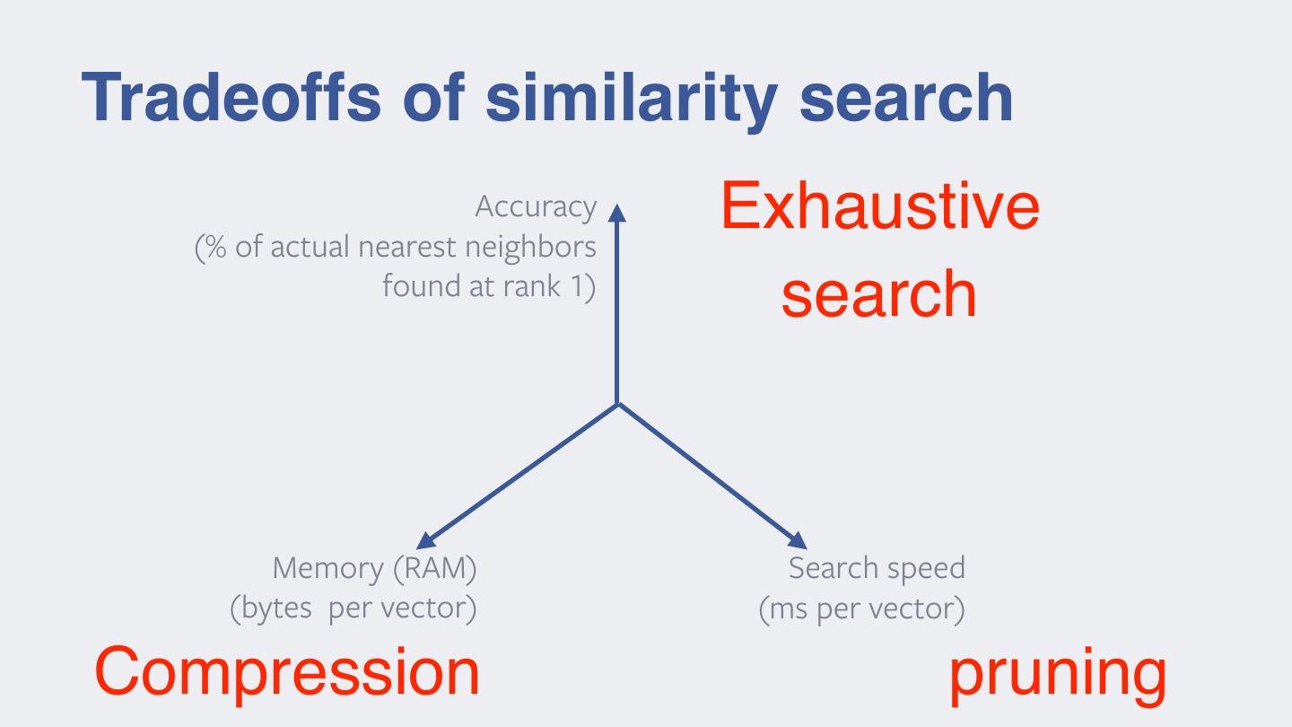
13 .Tradeoffs of similarity search 13 

14 .Tradeoffs of similarity search Accuracy (% of actual nearest neighbors Exhaustive found at rank 1) search Memory (RAM) Search speed (bytes per vector) (ms per vector) Compression pruning 

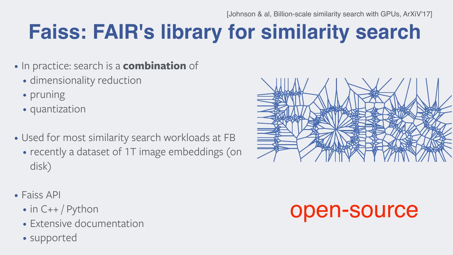
15 . [Johnson & al, Billion-scale similarity search with GPUs, ArXiV'17] Faiss: FAIR's library for similarity search • In practice: search is a combination of • dimensionality reduction • pruning • quantization • Used for most similarity search workloads at FB • recently a dataset of 1T image embeddings (on disk) • Faiss API • in C++ / Python • Extensive documentation open-source • supported 

16 . Compression [Product Quantization for Nearest Neighbor Search, Jégou, Douze, Schmid, PAMI 11] [Searching in one billion vectors: re-rank with source coding, Jégou, Tavenard, Douze, Amsaleg, ICASSP 11] [Large-scale image classification with trace-norm regularization, Harchaoui, Douze, Paulin, Dudik, Malick, CVPR 12] 16 

17 .Basic tool: vector quantization A lossy codec • Compress an embedding vector into a single integer 1 5 d R ! {1, ..., k} 2 4 3 

18 . Searching with quantizers • Consider asymmetric setting • no constraint on storage of query • keep full query vector, encode q(x) = q(y) database vectors A • Distance estimator S • reproduction value of the quantizer: centroid symmetric case asymmetric case Fig. 2. Illustration of the symmetric and asymmetric distance computation. • approximate distance The distance d(x, y) is estimated with either the distance d(q(x), q(y)) (left) or the distance d(x, q(y)) (right). The mean squared error on the distance is ve on average bounded by the quantization error. T kx yk ⇡ kx q(y)k d • approximate nearest neighbor usage of storing the centroids (k ⇤ ⇥ D floating point values), which further reduces the efficiency if the centroid look-up table does no longer fit in cache memory. In the case where argmini kx q(yi )k m = 1, we can not afford using more than 16 bits to keep this cost tractable. Using k ⇤ = 256 and m = 8 is often a w • for a given query x, there are k possible distances -> precompute! reasonable choice. 1 

19 . An extension: product quantization q1 q2 q3 q4 q1(y1) q2(y2) q3(y3) q4(y4) • reconstruction value: concatenation of centroids 1 m y ⇡ [q1 (y ), ..., qm (y )] • distance computation: distance is additive m X 2 j j 2 kx yk ⇡ kx qj (y )k j=1 • precompute m look-up tables 

20 .[Jégou & al, Product quantization for nearest neighbor search, PAMI'11] Sizes & flops no compression vector quantizer product quantizer code size d log2(k) m*log2(k) quantization N/A k*d k*d cost distance d multiply-adds one look-up, one add m look-ups, m adds computation cost number of N/A k k^m distinct values GOOD! 

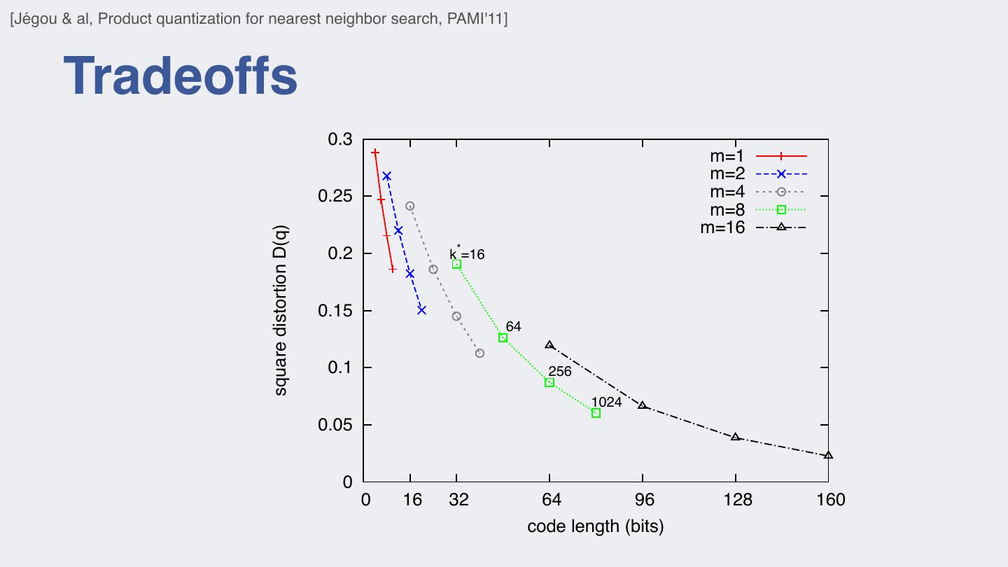
21 . M EMORY USAGE OF THE CODEBOOK AND ASSIGNMENT COMPLEXITY FOR [Jégou & al, Product quantization for nearest neighbor search, PAMI'11] . HKM IS PARAMETRIZED BY TREE HEIGHT l vector, for example the DIFFERENT QUANTIZERS producing 64-bits codes, AND THE BRANCHING FACTOR bf . Tradeoffs ntains k = 2 centroids. 64 oyd’s algorithm or even uired and the complexity 0.3 m=1 ral times k. It is even m=2 m=4 point values representing 0.25 m=8 m=16 square distortion D(q) solution to address these 0.2 k*=16 n source coding, which ponents to be quantized 0.15 64 omponents can be quan- e). The input vector x is 0.1 256  j  m of dimension 1024 e of m. The subvectors 0.05 tinct quantizers. A given ws: 0 0 16 32 64 96 128 160 1 u1 (x)), ..., qm (um (x) , code length (bits) 

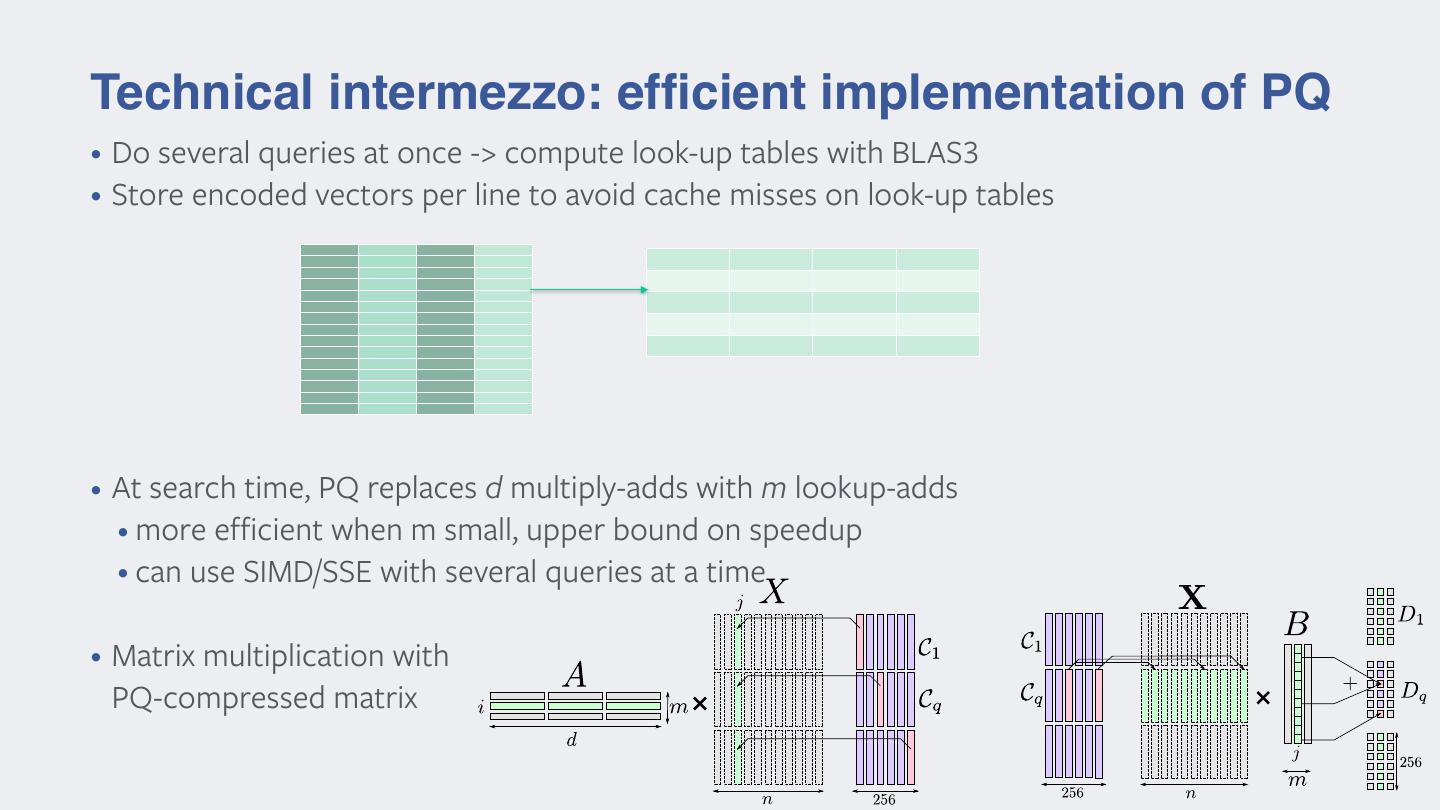
22 .Technical intermezzo: efficient implementation of PQ • Do several queries at once -> compute look-up tables with BLAS3 • Store encoded vectors per line to avoid cache misses on look-up tables • At search time, PQ replaces d multiply-adds with m lookup-adds • more efficient when m small, upper bound on speedup • can use SIMD/SSE with several queries at a time • Matrix multiplication with PQ-compressed matrix × × 

23 . Pruning [Product Quantization for Nearest Neighbor Search, Jégou, Douze, Schmid, PAMI 11] [The inverted multi-index, Babenko, Lempitsky, CVPR 12] 23 

24 .Exploring only a subset of the dataset • split the space into k clusters of vectors • usually clusters are defined by k-means • assign vectors to nearest centroid • index = inverted list structure • maps centroid id -> list of vectors assigned to it • search procedure • 1. find np << k nearest centroids to query vector • 2. scan the lists corresponding to the np centroids • any speedup in basic similarity search benefits to stage 1! 

25 . To get a good vector approximation, K should be large (K = 264 for a 64 bit code). For such large values of K, learning a K- Multiple quantization levels means codebook is not tractable, neither is the assignment of the vectors to their nearest centroids. To address this issue, [5] uses a product quantizer, for which there is no need to explicitly enumer- ate the centroids. A vector y ∈ Rd is first split into m subvectors y 1 , ..., y m ∈ Rd/m . A product quantizer is then defined as a func- • Coarse quantizer + residual quantizer tion ! 1 1 m m " qc (y) = q (y ), ..., q (y ) , (4) dr dc • reproduction value: which maps the input vector y to a tuple of indices by separately quantizing the subvectors. Each individual quantizer q (.) has K j s reproduction values, learned by K-means. To limit the assignment y ⇡ O(m complexity, qc (y) × K ),+K qisfset(yto a small s qcvalue s (y))(e.g. K =256). s However, the set of K centroids induced by the product quantizer qc (.) is large, as K = (Ks )m . The squared distances in Equation 2 • are computed using the decomposition IVFADC: coarse = k-means quantizer, fine = product quantizer Fig. 1. Illustration of the proposed refinement process. For database vector y, the distance d (x, y) = d(x, q (y)) is comp # c c 2 dc (x, y) = #x − qc (y)# =2 #xj − qj (y j )#2 , (5) • inverted file structure to build the short-list of potential nearest neighbors. For select j=1,...,m vectors, the distance is re-estimated by d (x, y), which is obta r j th by computing the distance between y and its improved approx where y is the j subvector of y. The squared distances in the sum tion dr = qc (y) + qr (y − qc (y)). are read from look-up tables. These tables are constructed on-the-fly for a given query, prior to the search in the set of quantization codes, estimated distances. This is done by encoding the residual ve from each subvector xj and the ks centroids associated with the cor- r(y) using another product quantizer qr defined by its reproduc responding quantizer qj . The complexity of the table generation is values Cr : O(d × Ks ). When Ks % n, this complexity is negligible compared qr (r(y)) = arg min #r(y) − c#2 , c∈Cr • At search time: select to the summation cost of O(d × n) in Equation 2. subset of centroids This approximate nearest neighbor method implicitly sees multi- where the product quantizer q (.) is learned on an independent s r residual vectors. Similar to q (.), the set of reproduction values • visit only points in the Voronoi as a vectorcells (inverted lists) c dimensional indexing approximation problem: a database never exhaustively listed, as all operations are performed using vector y can be decomposed as product space decomposition. argmini kx qc (yThe i ) coded qf (y q (y ))k • within inverted list: normal PQ y = qsearch (y) + r(y), c (6) i c i residual vector can be seen as the “least signifi bits”, except that the term “bits” usually refers to scalar quan query PQ codes tion. An improved estimation ŷ of y is the sum of the approxima 

26 . State of the art for large datasets . The residual vectors are encoded, producing the codes Method ADC ! m 0 recall@1 @10 @100 time/query 0.075 0.274 0.586 5.626 qr (yi − qc (yi )) associated with all the indexed vectors. 8! 0.258 0.683 0.951 5.686 • . Thea query ching Extended residual to vectors vector 3 quantization are encoded, x proceeds levels as follows: [ICASSP producing the codes11] Method ADC+R m 16 recall@1 0.434 @10 @100 0.895 0.982 time/query 5.692 q (y r i − q• more (y c i )) hyperparams... associated with all the indexed vectors. ADC 0 32 0.075 0.656 0.274 0.970 0.586 0.985 5.626 5.689 . The ADC distance estimation is used to generate a list L of ! • tests on 1B SIFT vectors IVFADC 8 0 0.258 0.088 0.683 0.372 0.951 0.733 5.686 0.074 k hypotheses. The selected vectors minimize the estimator ADC+R 16 0.434 0.895 0.962 0.982 5.692 ching a query BIGANN vector x dataset proceeds as follows: 8 0.262 0.701 0.116 of Equation 5, which is computed directly in the compressed 32 0.656 0.970 0.985 5.689 . domain The ADC [5].distance estimation is used to generate a list L of IVFADC+R 16 0.429 0.894 0.982 0.119 k! hypotheses. • Coarse quantizer The selected can be vectorsa PQ minimize the estimator IVFADC 0 32 0.088 0.630 0.372 0.977 0.733 0.983 0.074 0.120 . For each vector yi ∈ L, the approximate vector ŷi is explic- 8 0.262 0.701 0.962 0.116 of Equation • 5, which algorithm is to computed enumerate directly nearest in the compressed neighbors with PQ itly reconstructed using the first approximation qc (yi ) and the IVFADC+R Table 1. 16 and0.429 Performance efficiency 0.894 measured 0.982 on 1 0.119 billion vectors, domain [5]. • [Thevector inverted multi-index, Babenko, Lempitsky, CVPR 12] coded residual qr (y i ), see Equation 9. The squared m=8. The query 32 is measured time 0.630 in 0.977 seconds 0.983 per query. 0.120 The timings . distance For each estimator vector yi d(x, ∈ L,ŷithe 2 ) is approximate subsequently vector ŷi is explic- computed. validate the limited impact of the re-ranking stage on efficiency. itly reconstructed • Improve using the first sub-vector approximation allocation by qc (yi ) and optimizing the the rotation Table 1. Performance and efficiency measured on 1 billion vectors, . The vectors of L associated with the k smallest refined dis- coded residual • vectorPQ Alternate qr computation (yi ), see Equation and 9. The squared estimation of the rotation m=8. matrix The query time is measured in seconds per query. The timings tances are computed. 2 distance estimator d(x, ŷ i ) is subsequently computed. [Optimized Product Quantization for Approximate Nearest validate the limited Neighbor impact Search, ofsmaller the re-ranking Tiezheng Ge, Kaimingstage He, on efficiency. Qifa Ke,10M, Jian ..., On output, we obtain a re-ranked list of k approximate nearest vector. The groundtruth for sets (n=1M, 2M, 5M, . The vectorsSun, of LCVPR associated 13] with! the k smallest refined dis- 200M vectors) is also provided. As our own approach does not re- hbors. The choice of the number k of vectors in the short-list tances are computed. ! ! quire many training vectors, we only used the first million vectors nds on parameters m, m , k and on the distribution of the vec- vector. from theThe groundtruth learning set. for All smaller sets measurements (n=1M, 2M, (accuracy 5M, and 10M, ..., timings) On order •for In output, wetheobtain Optimize a re-ranked search post-verificationspeedlist — of k approximate scheme nearest to have a negligible hbors. The choice of the number ! ! of vectors in the short-list k 200M were vectors) over averaged is also the provided. 1000 first As our own approach does not re- queries. • Storingset plexity, we typically PQthe ! look-up ratio ktables ! /k to in2. registers quire many training vectors, we only used the first million vectors nds on parameters m, m , k and on the distribution [André, Kermarrec , Le Scouarnec Quicker ADC : Unlocking of the vec- the hidden potential of Product Quantization with SIMD, In order for the post-verification scheme to have a negligible from the learning set. All measurements (accuracy and timings) Non exhaustive PAMI’19] variant 4.2. Evaluation protocol plexity, we typically set the ratio k /k to 2. ! were averaged over the 1000 first queries. 

27 .Results on 1B vectors Based on Inverted multi-index and Polysemous codes BIGANN academic benchmark • 16 bytes + id per vector • Almost x10 faster than best reported results • Typically, <0.5 ms per query per thread 

28 .Billion-scale search QPS Non-exhaustive search + product quantization 10k • 1k-10k queries per 1k second (32 threads) 100 • accuracy 50% at 32 bytes 10 1 

29 . Searching with neighborhood graphs 29