Lecture 3 数据流与循环

1 .CSC D70: Compiler Optimization Dataflow-2 and Loops Prof. Gennady Pekhimenko University of Toronto Winter 2018 The content of this lecture is adapted from the lectures of Todd Mowry and Phillip Gibbons

2 .Refreshing from Last Lecture 2 Reaching definitions Live variables

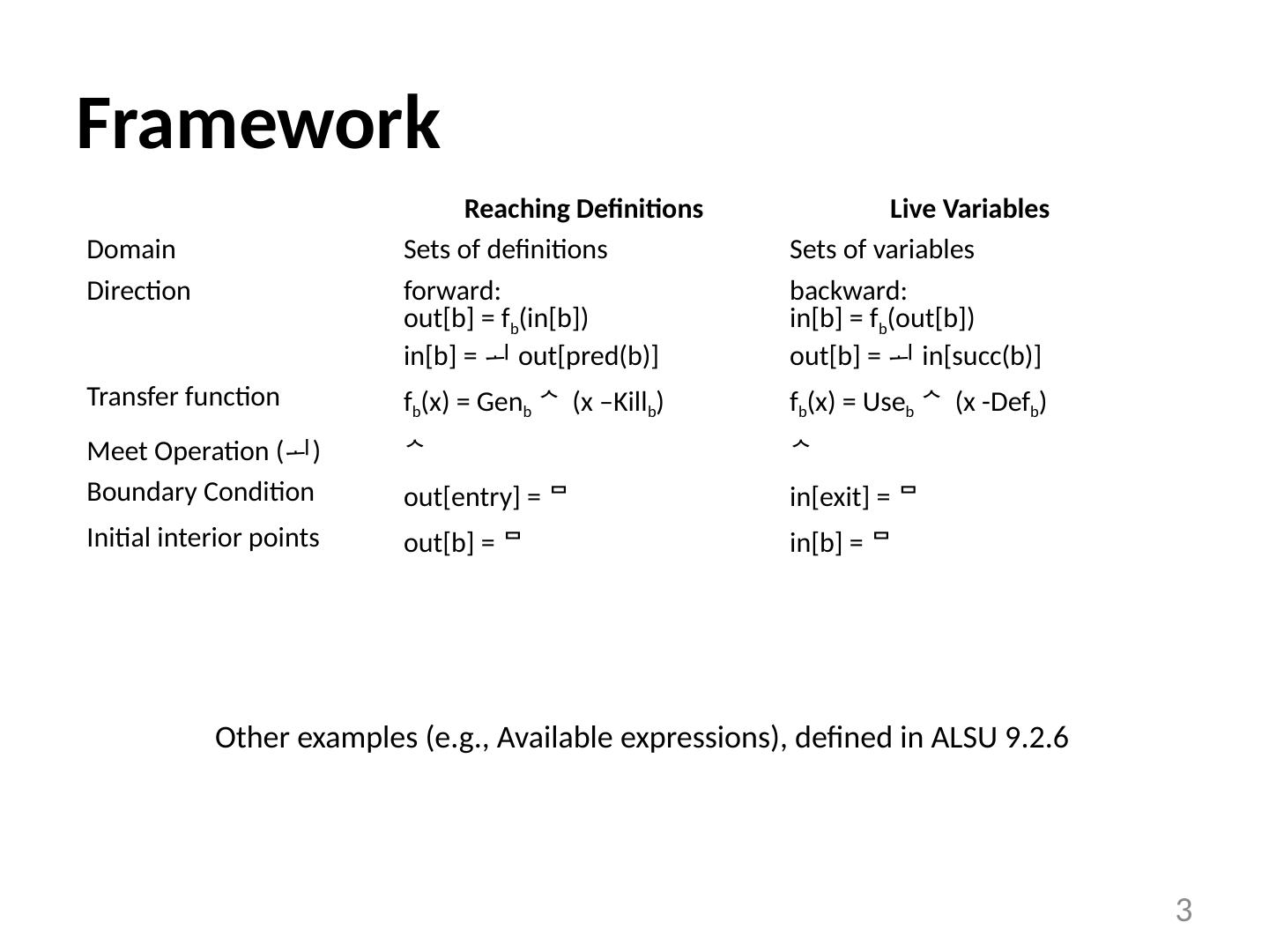
3 .Framework Reaching Definitions Live Variables Domain Sets of definitions Sets of variables Direction forward: out[b] = f b (in[b]) in[b] =  out[ pred (b)] backward: in[b] = f b (out[b]) out[b] =  in[ succ (b)] Transfer function f b (x) = Gen b  (x –Kill b ) f b (x) = Use b  (x -Def b ) Meet Operation ( )   Boundary Condition out[entry] =  in[exit] =  Initial interior points out[b] =  in[b] =  3 Other examples (e.g., Available expressions), defined in ALSU 9.2.6

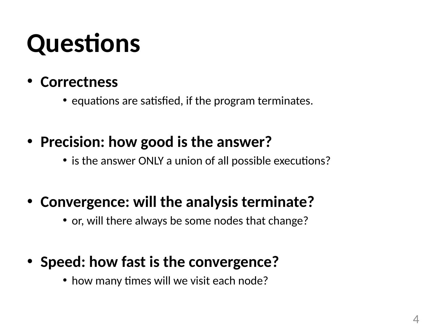
4 .Questions Correctness equations are satisfied, if the program terminates. Precision: how good is the answer? is the answer ONLY a union of all possible executions? Convergence: will the analysis terminate? or, will there always be some nodes that change? Speed: how fast is the convergence? how many times will we visit each node? 4

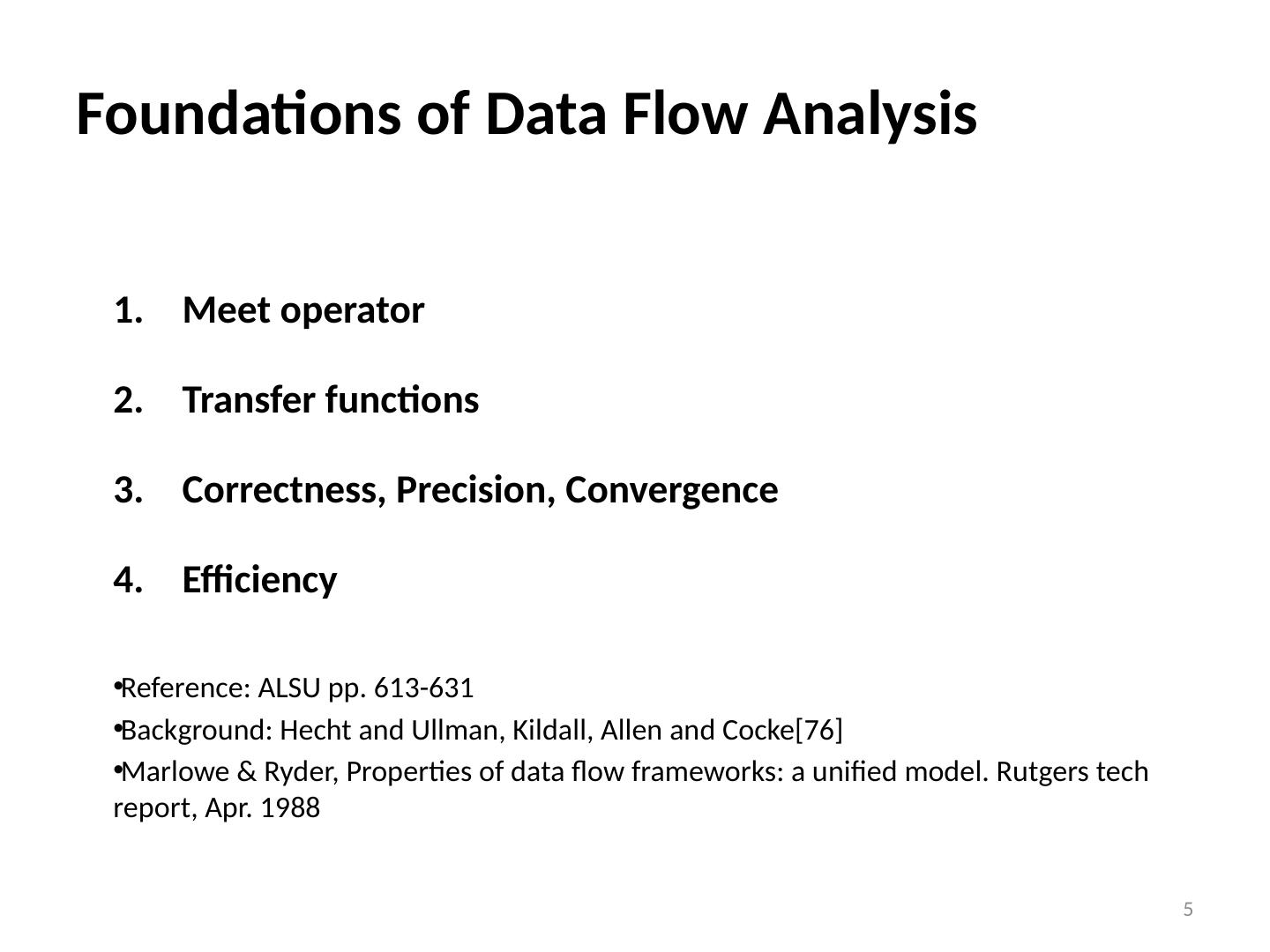
5 .Foundations of Data Flow Analysis Meet operator Transfer functions Correctness, Precision, Convergence Efficiency Reference: ALSU pp. 613-631 Background: Hecht and Ullman , Kildall , Allen and Cocke [76] Marlowe & Ryder, Properties of data flow frameworks: a unified model. Rutgers tech report, Apr. 1988 5

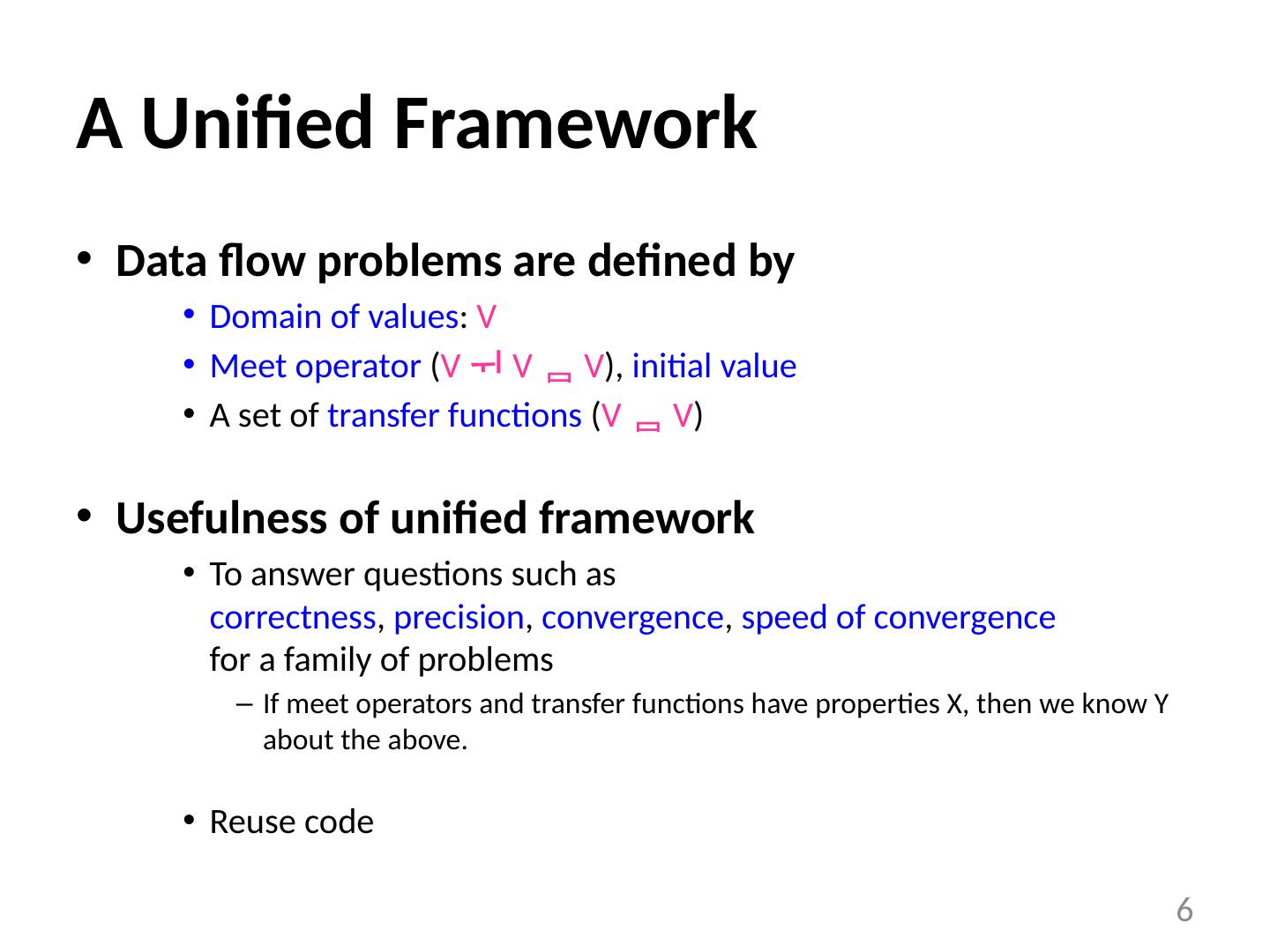
6 .A Unified Framework Data flow problems are defined by Domain of values : V Meet operator ( V  V  V ), initial value A set of transfer functions ( V  V ) Usefulness of unified framework To answer questions such as correctness , precision , convergence , speed of convergence for a family of problems If meet operators and transfer functions have properties X, then we know Y about the above. Reuse code 6

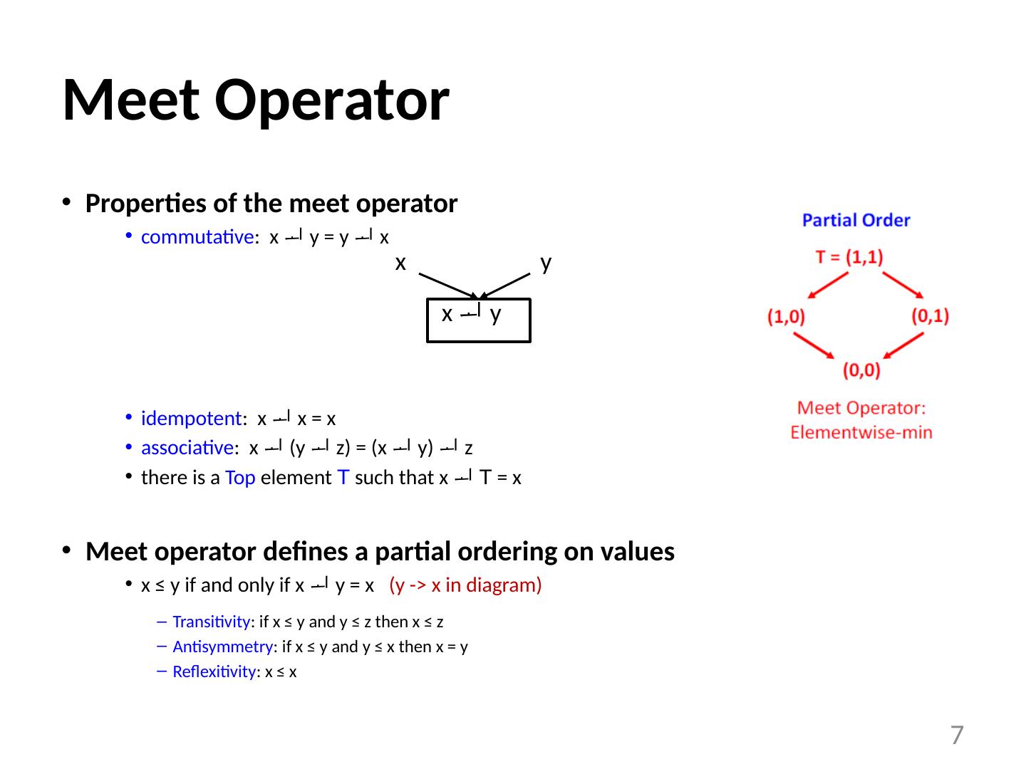
7 .Meet Operator Properties of the meet operator commutative : x  y = y  x idempotent : x  x = x associative : x  (y  z) = (x  y)  z there is a Top element T such that x  T = x Meet operator defines a partial ordering on values x ≤ y if and only if x  y = x (y -> x in diagram) Transitivity : if x ≤ y and y ≤ z then x ≤ z Antisymmetry : if x ≤ y and y ≤ x then x = y Reflexitivity : x ≤ x 7 x y x  y

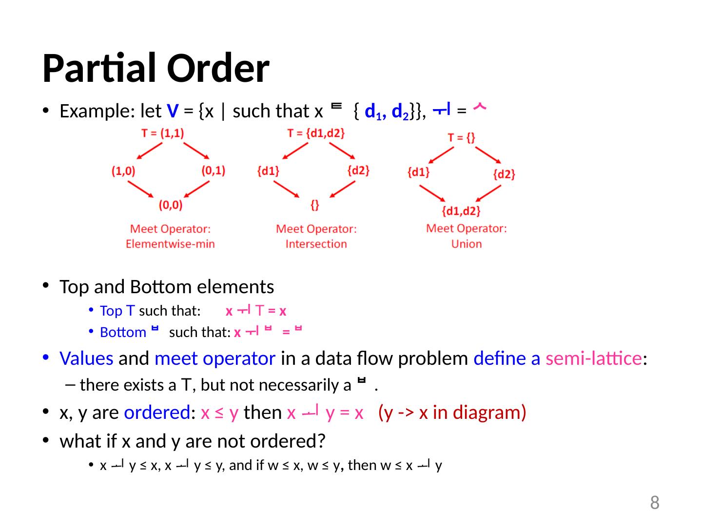
8 .Partial Order Example: let V = {x | such that x  { d 1 , d 2 }},  =  Top and Bottom elements Top T such that: x  T = x Bottom  such that: x   =  Values and meet operator in a data flow problem define a semi-lattice : there exists a T , but not necessarily a  . x, y are ordered : x ≤ y then x  y = x (y -> x in diagram) what if x and y are not ordered? x  y ≤ x, x  y ≤ y, and if w ≤ x, w ≤ y , then w ≤ x  y 8

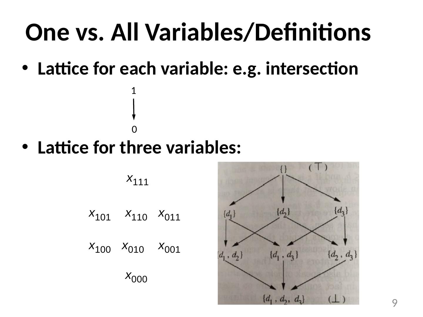
9 .One vs. All Variables/Definitions Lattice for each variable: e.g. intersection Lattice for three variables: 9 1 0

10 .Descending Chain Definition The height of a lattice is the largest number of > relations that will fit in a descending chain. x 0 > x 1 > x 2 > … Height of values in reaching definitions? Important property: finite descending chain Can an infinite lattice have a finite descending chain? Example: Constant Propagation/Folding To determine if a variable is a constant Data values undef , ... -1, 0, 1, 2, ..., not-a-constant 10 Height n – number of definitions yes

11 .Transfer Functions Basic Properties f : V  V Has an identity function There exists an f such that f (x) = x, for all x. Closed under composition if f 1 , f 2  F , then f 1  f 2  F 11

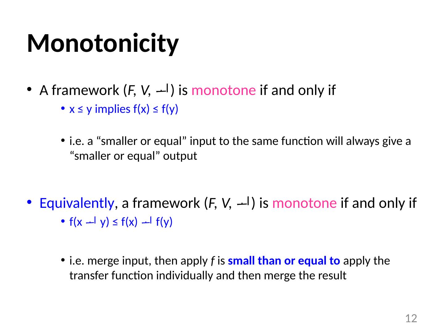
12 .Monotonicity A framework ( F, V,  ) is monotone if and only if x ≤ y implies f(x) ≤ f(y) i.e. a “smaller or equal” input to the same function will always give a “smaller or equal” output Equivalently , a framework ( F, V,  ) is monotone if and only if f(x  y) ≤ f(x)  f(y) i.e. merge input, then apply f is small than or equal to apply the transfer function individually and then merge the result 12

13 .Example Reaching definitions: f(x) = Gen  (x - Kill) ,  =  Definition 1: x 1 ≤ x 2 , Gen  (x 1 - Kill) ≤ Gen  (x 2 - Kill) Definition 2: (Gen  (x 1 - Kill) )  (Gen  (x 2 - Kill) ) = (Gen  ((x 1  x 2 ) - Kill)) Note: Monotone framework does not mean that f(x) ≤ x e.g., reaching definition for two definitions in program suppose: f x : Gen x = {d 1 , d 2 } ; Kill x = {} If input(second iteration) ≤ input(first iteration) result(second iteration) ≤ result(first iteration) 13

14 .Distributivity A framework ( F, V,  ) is distributive if and only if f(x  y) = f(x)  f(y) i.e. merge input, then apply f is equal to apply the transfer function individually then merge result Example: Constant Propagation is NOT distributive 14 a = 2 b = 3 a = 3 b = 2 c = a + b

15 .Data Flow Analysis Definition Let f 1 , ..., f m :  F , where f i is the transfer function for node i f p = f n k  …  f n 1 , where p is a path through nodes n 1 , ..., n k f p = identify function , if p is an empty path Ideal data flow answer: For each node n:  f p i ( T ) , for all possibly executed paths p i reaching n . But determining all possibly executed paths is undecidable 15 x = 0 x = 1 if sqrt (y) >= 0

16 .Meet-Over-Paths (MOP) Error in the conservative direction Meet-Over-Paths (MOP): For each node n: MOP( n ) =  f p i ( T ) , for all paths p i reaching n a path exists as long there is an edge in the code consider more paths than necessary MOP = Perfect-Solution  Solution-to-Unexecuted-Paths MOP ≤ Perfect-Solution Potentially more constrained, solution is small hence conservative It is not safe to be > Perfect-Solution! Desirable solution: as close to MOP as possible 16

17 .MOP Example 17

18 .Solving Data Flow Equations Example: Reaching definitions out[entry] = {} Values = {subsets of definitions} Meet operator :  in[b] =  out[ p ], for all predecessors p of b Transfer functions : out[b] = gen b  (in[b] - kill b ) Any solution satisfying equations = Fixed Point Solution ( FP ) Iterative algorithm initializes out[b] to {} if converges, then it computes Maximum Fixed Point ( MFP ): MFP is the largest of all solutions to equations Properties: FP ≤ MFP ≤ MOP ≤ Perfect-solution FP, MFP are safe in(b) ≤ MOP(b) 18

19 .Partial Correctness of Algorithm If data flow framework is monotone , then if the algorithm converges, IN[b] ≤ MOP[b] Proof: Induction on path lengths Define IN[entry] = OUT[entry] and transfer function of entry = Identity function Base case: path of length 0 Proper initialization of IN[entry] If true for path of length k , p k = ( n 1 , ..., n k ), then true for path of length k+1: p k +1 = ( n 1 , ..., n k+1 ) Assume: IN[ n k ] ≤ f n k-1 ( f n k-2 (... f n 1 (IN[entry]))) IN[n k+1 ] = OUT[ n k ]  ... ≤ OUT[ n k ] ≤ f n k (IN[ n k ]) ≤ f n k-1 ( f n k-2 (... f n 1 (IN[entry]))) 19

20 .Precision If data flow framework is distributive ,then if the algorithm converges, IN[b] = MOP[b] Monotone but not distributive: behaves as if there are additional paths 20 a = 2 b = 3 a = 3 b = 2 c = a + b

21 .Additional Property to Guarantee Convergence Data flow framework ( monotone ) converges if there is a finite descending chain For each variable IN[b], OUT[b], consider the sequence of values set to each variable across iterations : if sequence for in[b] is monotonically decreasing sequence for out[b] is monotonically decreasing (out[b] initialized to T ) if sequence for out[b] is monotonically decreasing sequence of in[b] is monotonically decreasing 21

22 .Speed of Convergence Speed of convergence depends on order of node visits Reverse “direction” for backward flow problems 22

23 .Reverse Postorder Step 1: depth-first post order main() { count = 1; Visit( root ); } Visit(n) { for each successor s that has not been visited Visit(s); PostOrder (n) = count ; count = count+1 ; } Step 2: reverse order For each node i rPostOrder = NumNodes - PostOrder ( i ) 23

24 .Depth-First Iterative Algorithm (forward) input: control flow graph CFG = (N, E, Entry, Exit) /* Initialize */ out[entry] = init_value For all nodes i out[ i ] = T Change = True /* iterate */ While Change { Change = False For each node i in rPostOrder { in[ i ] =  (out[p]), for all predecessors p of i oldout = out[ i ] out[ i ] = f i (in[ i ]) if oldout  out[ i ] Change = True } } 24

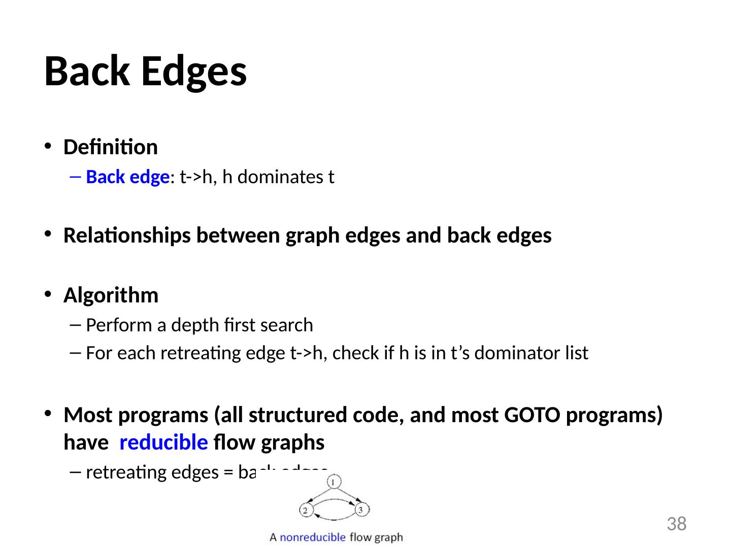
25 .Speed of Convergence If cycles do not add information information can flow in one pass down a series of nodes of increasing order number: e.g., 1 -> 4 -> 5 -> 7 -> 2 -> 4 ... passes determined by number of back edges in the path essentially the nesting depth of the graph Number of iterations = number of back edges in any acyclic path + 2 (2 are necessary even if there are no cycles) What is the depth? corresponds to depth of intervals for “reducible” graphs in real programs: average of 2.75 25

26 .A Check List for Data Flow Problems Semi-lattice set of values meet operator top, bottom finite descending chain? Transfer functions function of each basic block monotone distributive? Algorithm initialization step (entry/exit, other nodes) visit order: rPostOrder depth of the graph 26

27 .Conclusions Dataflow analysis examples Reaching definitions Live variables Dataflow formation definition Meet operator Transfer functions Correctness, Precision, Convergence Efficiency 27

28 .CSC D70: Compiler Optimization Loops Prof. Gennady Pekhimenko University of Toronto Winter 2018 The content of this lecture is adapted from the lectures of Todd Mowry and Phillip Gibbons

29 .What is a Loop? Goals: Define a loop in graph-theoretic terms (control flow graph) Not sensitive to input syntax A uniform treatment for all loops: DO, while, goto’s Not every cycle is a “loop” from an optimization perspective Intuitive properties of a loop single entry point edges must form at least a cycle 29 Is this a loop? Is this a loop?