Importance Sampling for Fair Pol

1 . Importance Sampling for Fair Policy Selection Shayan Doroudi Philip S. Thomas Emma Brunskill Computer Science Department Computer Science Department Computer Science Department Carnegie Mellon University Carnegie Mellon University Stanford University Pittsburgh, PA 15213 Pittsburgh, PA 15213 Stanford, CA 94305 shayand@cs.cmu.edu philipt@cs.cmu.edu ebrun@cs.stanford.edu Abstract unfairness can occur in both the on-policy and off-policy settings. We further show that in the off-policy set- ting, using importance sampling for policy selection can We consider the problem of off-policy policy be unfair in practically relevant settings. In particular, selection in reinforcement learning: using his- we show that IS can favor myopic policies—policies torical data generated from running one pol- that obtain less total reward, but which obtain it early icy to compare two or more policies. We show in an episode—as well as favoring policies that pro- that approaches based on importance sampling duce shorter trajectories. Although IS is an unbiased can be unfair—they can select the worse of estimator, this unfairness arises because policy selec- two policies more often than not. We give two tion involves taking a maximum over estimated quanti- examples where the unfairness of importance ties. Depending on the distribution of estimates, impor- sampling could be practically concerning. We tance sampling may systematically favor policies that are then present sufficient conditions to theoreti- worse in expectation. cally guarantee fairness and a related notion of safety. Finally, we provide a practical impor- We then present two new approaches for avoiding un- tance sampling-based estimator to help miti- fairness when using importance sampling for policy se- gate one of the systematic sources of unfair- lection. First, we give sufficient conditions under which ness resulting from using importance sampling using importance sampling for policy selection is fair, for policy selection. and provide algorithms that guarantee a related notion of safety. We also describe how our approach to guarantee- ing fairness and safety is related to the notions of power 1 INTRODUCTION analysis and statistical hypothesis testing. Although of theoretical interest, the reliance of this approach on con- In this paper, we consider the problem of off-policy pol- servative concentration inequalities limits its practicality. icy selection: using historical data generated from run- Thus, in our second approach, we introduce a new prac- ning one policy to compare two or more policies. Off- tical IS-based estimator that lacks the theoretical prop- policy policy selection methods can be used, for exam- erties of our first approach, but which can help mitigate ple, to decide which policy should be deployed when two unfairness due to differing trajectory lengths. or more batch reinforcement learning (RL) algorithms Although there is significant literature surrounding re- suggest different policies or when a data-driven policy is ducing the variance and mean squared error of off-policy compared to a policy designed by a human expert. The policy evaluation methods that use IS-based estimators primary contribution of this paper is that we show that (Powell and Swann, 1966; Dud´ık et al., 2011; Jiang and the importance sampling (IS) estimator (Precup et al., Li, 2016; Thomas and Brunskill, 2017), other challenges 2000), which lies at the foundation of many policy selec- associated with off-policy policy selection, such as fair- tion and policy search algorithms (Mandel et al., 2014; ness, have not been explored in the literature. Similar Levine and Koltun, 2013; Thomas et al., 2015b), is often notions of fairness have recently been proposed in the unfair when used for policy selection: when comparing online RL setting, where an algorithm is fair if it never two policies, the worse of the two policies may be re- takes a worse action with higher probability than a bet- turned more than half the time. ter action Jabbari et al. (2017). This is similar to our After formalizing our notion of fairness, we show that notion of fairness in the offline RL setting, where an al- 

2 .gorithm is fair if it does not choose a worse policy with where Ri,t and Ti denote the reward of τi at time t and higher probability than the best candidate policy. How- the length of τi respectively. ever, the issues surrounding fairness in the two settings are different due to the different nature of each setting. 2.2 IMPORTANCE SAMPLING By introducing a notion of fairness for policy selection and highlighting some limitations of existing IS-based In this paper, we primarily focus on off-policy policy approaches, we hope to motivate further work on devel- evaluation and selection. Specifically, we focus on esti- oping practical and fair policy selection algorithms. mators that use importance sampling. Model-based off- policy estimators tend to have lower variance than IS- 2 BACKGROUND based estimators, but at the cost of being biased and asymptotically incorrect (not consistent estimators of We consider sequential decision making set- V π ) (Mandel et al., 2014). In contrast, IS-based estima- tings in stochastic domains. In such do- tors can provide unbiased estimates of the value. There mains, an agent interacts with the environ- has been significant interest in using IS-based techniques ment, and in doing so, it generates a trajectory, in RL for policy evaluation (Precup et al., 2000; Jiang τ (O0 , A1 , R1 , O1 , A2 , R2 , . . . , AT , RT , OT ), which and Li, 2016; Thomas and Brunskill, 2016), as well as is a sequence of observations, actions, and rewards, growing recent interest in using it for policy selection with trajectory length T . The observations and re- (Mandel et al., 2014) and the related problems of policy wards are generated by the environment according to a search and policy gradient optimization (Jie and Abbeel, stochastic process—such as a Markov decision process 2010; Levine and Koltun, 2013; Thomas et al., 2015b; (MDP) or partially observable Markov decision process Wang et al., 2016). (POMDP)—that is unknown. The agent chooses actions The IS estimator (Precup et al., 2000) is given according to a stochastic policy π, which is a conditional by: VˆISπe 1 n Ti n i=1 wi t=1 Ri,t , where wi probability distribution over actions At given the partial Ti πe (ai,t |τi,1:t−1 ) trajectory τ1:t−1 (O0 , A1 , R1 , O1 , A2 , R2 , . . . , Ot−1 ) t=1 πb (ai,t |τi,1:t−1 ) . The IS estimator is an un- of prior observations, actions, and rewards. The value biased and strongly consistent estimator of V πe if of a policy π, V π , is the expected sum of rewards when πe (a|τ1:t−1 ) = 0 for all actions, a, and partial tra- T jectories, τ1:t−1 , where πb (at |τ1:t−1 ) = 0. How- the policy is used: V π E t=1 Rt τ ∼ π , where ever, VˆISπe often has high variance. The weighted τ ∼ π means that the actions of τ are sampled according importance sampling (WIS) estimator, VˆWIS πe to π. The agent’s goal is to find and execute a policy 1 n Ti with a large value. n i=1 wi i=1 wi t=1 Ri,t , is a variant of the IS esti- mator that often has much lower variance, but which is In this paper, we consider offline (batch) reinforcement not an unbiased estimator of V πe . learning (RL) where we have a batch of data, called his- torical data, that was generated from some known be- 3 FAIR POLICY SELECTION havior policy πb . We are interested in the problem of batch policy selection: identifying a good policy for use A policy selection algorithm is given a set of candidate in the future. This typically involves policy evaluation or policies and must choose one of the policies for use in the estimating the value of a policy πe using the historical future. Any policy evaluation algorithm (i.e., estimator) data that was generated from the behavior policy πb . If can be converted to a policy selection algorithm by sim- πe = πb this is known as on-policy policy evaluation. ply evaluating each policy using the estimator, and then Otherwise it is known as off-policy policy evaluation. selecting the policy that has the largest estimated value. Thus we can use the Monte Carlo estimator for on-policy 2.1 ON-POLICY POLICY EVALUATION policy selection, and we can use the IS or WIS estimators for off-policy policy selection. Although we are primarily interested in the off-policy setting, i.e., the setting where πb = πe , we will also dis- There are two natural properties we would like in a batch cuss the problem of on-policy policy evaluation. This policy selection algorithm: problem arises, for example, when running a random- • Consistency: In the limit as the amount of historical ized control trial or A/B test to compare two policies. In data goes to infinity, the algorithm should always this case, the value of each policy is directly estimated select the policy that has the largest value. by running it to generate n trajectories, τ1 , τ2 , . . . , τn , and then estimating the policy’s performance using the • Fairness: With any amount of historical data, the n Ti Monte Carlo estimator: VˆMC,n πe 1 n i=1 t=1 Ri,t , probability that the algorithm selects a policy with 

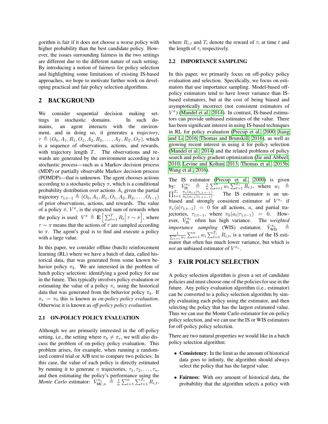
3 . the largest value should be greater than the proba- Table 1: The probability of each action under π1 and π2 bility that it selects a policy that does not have the for the example domain where Monte Carlo estimation is largest value. When choosing between two poli- unfair. Rewards, R, are deterministic. cies, this implies that the algorithm should choose the better policy at least half the time.1 a1 (R = 0) a2 (R = r) a3 (R = 1) Exploring and ensuring the fairness of (IS-based) pol- π1 0 1 0 icy selection algorithms is the focus of this paper. There π2 1−p 0 p has been recent interest on combining model-based es- timators and IS-based estimators (Jiang and Li, 2016; π2 , in a multi-armed bandit (MAB) domain with three Thomas and Brunskill, 2016), however as both model- actions a1 , a2 , and a3 with rewards and probabilities as based estimators and (as we will show) IS-based estima- described in Table 1. Notice that V π1 = r and V π2 = p. tors are unfair, it is easy to show that these new estimators So, if r < p, then V π1 < V π2 . However, notice that must also be unfair. Therefore, we restrict our attention using one trajectory (n = 1), the Monte Carlo estima- to the standard IS and WIS estimators. tor is unfair with respect to V if r < p < 0.5 since Pr(VˆMC,1 π1 ≤ VˆMC,1 π2 ) = p. We can similarly show that Before proceeding, we formally define a way to rank Monte Carlo policy selection is unfair using n trajecto- policies. Let the better-than operator B , be such that ries for n > 1, as long as r and p are sufficiently small. π1 B π2 is True if π1 is better than π2 and False otherwise, for some notion of “better”. For example, we can define V to order policies based on their values: 4 UNFAIRNESS OF IMPORTANCE π1 V π2 is True if V π1 > V π2 and False other- SAMPLING POLICY SELECTION wise. Define the optimal policy π ∗ in a policy class Π to be the policy where π ∗ B π for all π = π ∗ ∈ Π.2 We Unsurprisingly, importance sampling is also unfair with will now formally define fairness. respect to V . However, the unfairness of importance Definition 3.1. A policy selection algorithm that chooses sampling can be arbitrarily worse than the unfairness of policies from a policy class Π is fair with respect to a the Monte Carlo estimator, in that for any n, we can con- better-than operator B if whenever the algorithm out- struct a domain such that IS policy selection is unfair puts a policy, the probability that it outputs π ∗ is at least even though the Monte Carlo estimator will always pick as large as the probability that it will output any other the correct policy with even a single sample! We provide policy. The algorithm is strictly fair if the probability of one such example in Supplementary Material A. In this outputting policy π ∗ is strictly greater than the probabil- section, we present two examples that highlight how the ity of outputting any other policy. unfairness of importance sampling can arise in counter- intuitive ways in practically interesting settings, motivat- Notice that the probabilistic guarantee in this definition ing the importance of caring about satisfying fairness. conditions on when the algorithm outputs a policy. This allows for a policy selection algorithm that does not out- 4.1 IS FAVORS MYOPIC POLICIES put any policy in cases when it cannot determine which policy is better. Also, notice that the trivial policy selec- In the following example we show that even when com- tion algorithm that never outputs a policy is fair. How- paring two policies that are equally close to the behavior ever, ideally we want a policy selection algorithm that policy, importance sampling can still be unfair. In par- outputs a policy as often as possible while maintaining ticular, we show that using IS for policy selection could fairness. This is an important distinction: although we be biased in favor of myopic policies, which could be of want an algorithm that often outputs a policy, we re- significant practical concern. This may come up in prac- quire the algorithm to at least be fair. We now see that tical settings where we are interested in comparing more this seemingly straightforward property is not satisfied heuristic methods of planning (e.g., short look-ahead) to by even the most natural policy selection algorithms. full-horizon planning methods. If we have the correct model class, full horizon planning is expected to be op- We begin by showing that even Monte Carlo estimation timal, however it is both computationally expensive (so is unfair when used for on-policy policy selection. Sup- possibly not even tractable) and potentially sub-optimal pose we want to select the better of two policies, π1 and if our model class is incorrect (e.g., our state representa- 1 For simplicity, hereafter we assume that there are no two tion is inaccurate or the world is a POMDP but we are candidate policies that are equally good. modeling it as a MDP). Thus, we may be interested in 2 We assume such a best policy exists; however, for some comparing full-horizon planning (or an approximation reasonable better-than operators, this may not be true, as we thereof) to myopic planning, and the following exam- explore in Section 5.1. 

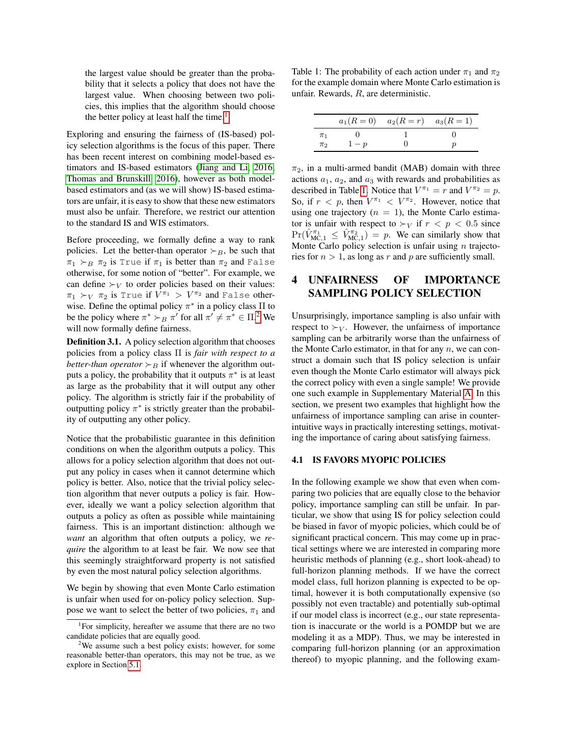
4 . R(aR ) = 0 R(aR ) = 0 R(aR ) = 0 R(aR ) = 0 R(aL ) = 1 s1 s2 s3 ... s10 R(aR ) = 10 R(aL ) = 1 R(aL ) = 1 R(aL ) = 1 Figure 1: Domain in Section 4.1. The agent is in a chain of length 10. In each state, the agent can either go right (aR ) which progresses the agent along the chain and gives a reward of 0 unless the agent is in s10 , in which case it gives a reward of 10 (and keeps the agent in the s10 ), or go left (aL ), which takes the agent back to state s1 and gives a reward of 1. with probability 0.5 with probability 0.5 R(aX ) = 1 R(aX ) = 1 R(aX ) = 0 R(aX ) = 0 R(aX ) = 0 s0 s1 s2 s0 s1 ... sL R(aY ) = 0 R(aY ) = 0 R(aY ) = 1 R(aY ) = 1 R(aY ) = 1 Figure 2: Domain in Section 4.2. The agent is placed uniformly at random in either a chain MDP of length 2 or a chain of length L. At each time step, action aX deterministically gives a reward of 1 to the agent if the agent is in the chain of length 2 and 0 otherwise, and action aY deterministically gives a reward of 1 to the agent if the agent is in the chain of length L and 0 otherwise. Both actions progress the agent along the chain. ple shows that IS can sometimes favor policies resulting suggest choosing the optimal policy. IS is unable to de- from myopic planning even when full horizon planning tect simple patterns that a model-based approach (or even is optimal. a human briefly looking at the data) would easily infer; this is the cost of having an evaluation technique that Consider the MDP given in Figure 1. Now suppose we places virtually no assumptions on policies. have data collected from a behavior policy πb that takes each action with probability 0.5 and all trajectories have 4.2 IS FAVORS SHORTER TRAJECTORIES length 200. We want to compare two policies: πmyopic which takes aL with probability 0.99 and aR with proba- Importance sampling can also systematically favor poli- bility 0.01, and πopt which takes aL with probability 0.01 cies that assign higher probability to shorter trajectory and aR with probability 0.99. (Note: the actual optimal lengths in domains where the length of each trajectory policy is to always take aR , for which πopt is a slightly may vary. This is a problem that could arise in many stochastic version.) Notice that the probability distribu- practical domains, for example domains where a user is tion of importance weights is the same for both πmyopic free to leave the system at any time, such as a student and πopt , so both are equally close to the behavior pol- solving problems in an educational game or a user chat- icy in terms of probability distributions over trajectories. ting with a dialogue system. In such systems, a bad pol- However, for datasets that are not large enough, the im- icy may cause a user to leave the system sooner resulting portance sampling estimate will be larger for πmyopic in a short trajectory, which makes it particularly prob- than for πopt , even though it is clearly the worse policy. lematic that importance sampling can favor policies that For example, when we have 1000 samples, (1) around assign higher probability to shorter trajectories. The fol- 60% of the time, the importance sampling estimate of lowing example shows that importance sampling can fa- πmyopic is larger than that of πopt , and (2) around 95% vor policies that generate shorter trajectories even when of the time, the weighted importance sampling estimate they are clearly worse. of πmyopic is larger than that of πopt . Thus both the IS and WIS estimators are unfair for policy selection. Consider the domain given in Figure 2. Now suppose we have data collected from a behavior policy πb that takes The reason IS is unfair in this case is because one policy each action with probability 0.5. We want to compare only gives high rewards in events that are unlikely under two policies: πX , which takes action aX with probabil- the behavior policy, and hence the behavior policy often ity 0.99, and πY , which takes action aY with probability does not see the high rewards of this policy as compared 0.99. Consider the case where L = 80. Clearly πY is to a myopic policy. However, note that these events are the better policy, because it incurs a lot of reward when still likely enough that we can build a model that would we encounter trajectories of length 80, while only los- 

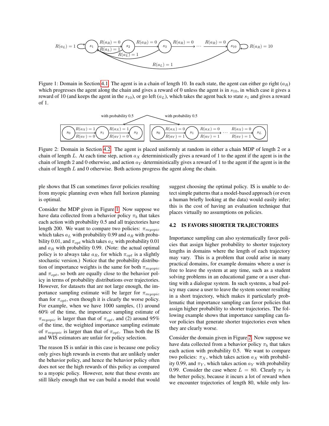
5 .Table 2: Median estimates, out of 100 simulations, of we would want to use if we want to find a policy where different estimators using 100 samples of πX and πY in we optimize our chance of beating a baseline in an ex- the domain in Section 4.2. periment or A/B test with n samples (i.e., obtaining a statistically significant result). Also, notice that we have VˆMC VˆIS VˆWIS a different better-than operator for each n, which is not necessarily related to the number of samples that we have πX 1.39 0.98 1.98 from our behavior policy πb . (For example, we may πY 39.52 0.010 0.020 have collected data from interactions with 1,000 users, ing out on a small reward when encountering the short but want to deploy a policy and expect one million users trajectories. Table 2 shows the median estimate, out of to use it; in that case we may want to be fair with respect 100 simulations, of the Monte Carlo estimator, as well to MC,106 .) We will use MC to refer to this notion of as the median IS and WIS estimates using 1000 samples better-than in general (even though it is not technically each. We find that while πY is, in actuality, much better, a better-than operator without specifying the number of IS essentially only weighs the shorter trajectories, so the samples). Of course, for this new better-than operator, estimates only reflect how well the policies do on those the Monte Carlo estimator is fair by definition. It is in- trajectories. WIS simply (almost) doubles the estimates teresting to note that if the distribution over the sum of because half of the samples have extremely low impor- rewards under the two policies are symmetric distribu- tance weights. So why does this occur? When using IS in tions (e.g., normal distributions), then the two better-than settings where trajectories can have varying lengths, the operators are equivalent. It may seem as though it is eas- importance weight of shorter trajectories can be much ier to satisfy fairness for importance sampling with re- larger than for longer trajectories, because for longer tra- spect to MC,n than with respect to V ; however, we jectories we are multiplying more ratios of probabilities will show below that, at least in some sense, this is not that are more often smaller than one. This happens even the case. However, we can present conditions where both if the policy we are evaluating is more likely to produce are satisfied simultaneously. We will henceforth consider longer trajectories than a shorter one (because there are and present results with respect to both notions of fair- exponentially many longer trajectories and so each in- ness (i.e., fairness with respect to V and fairness with dividual trajectory has an exponentially smaller weight respect to MC,n ). But we will first consider some coun- than an individual short trajectory). terintuitive properties of this new better-than operator. 5.1 FAIRNESS AND NON-TRANSITIVITY 5 A NEW KIND OF FAIRNESS It is a well-known result in probability theory that there The examples above illustrate that even the most straight- exists random variables X, Y , and Z such that Pr(X > forward way of evaluating policies could misguide some- Y ) > 0.5 and Pr(Y > Z) > 0.5, but Pr(Z > X) > one about which policy is actually better under the ob- 0.5 as well, indicating that comparing between random jective of maximizing the expected sum of reward. Al- variables in such a way is non-transitive (Trybuła, 1961; though we showed that off-policy policy selection using Gardner, 1970). We claim that this non-transitivity holds IS can be much less fair than doing on-policy Monte for the ordering induced by the MC,n operator as well. Carlo estimation, the fact that on-policy estimation is This is shown in Supplementary Material B. In fact, it also unfair suggests that perhaps we are using the wrong is possible that for any policy π, there is another policy measure of performance to construct our better-than op- π where MC,n (π , π) = True, meaning a best policy erators. The problem is that, even if π1 usually produces might not exist with respect to MC . trajectories with more reward than those produced by π2 , it could still be that V π1 < V π2 if there is a rare The good news is that over fifty years ago, trajectory with very large reward that is more likely un- Trybuła (1965) showed that for any m indepen- der π2 . It is therefore worth considering a different no- dent random variables X1 , . . . , Xm , min{Pr(X1 > tion of “better-than” that better captures which policy is X2 ), . . . Pr(Xm−1 > Xm ), Pr(Xm > X1 )} < 0.75. likely to perform better given a fixed and finite amount Thus, in order to avoid such non-transitivity, we motivate of historical data. This can be captured using the follow- a new kind of fairness: ing better-than operator, which we refer to as better-than with respect to Monte Carlo estimation: π1 MC,n π2 is Definition 5.1. An algorithm is transitively fair with re- True if Pr(VˆMC,nπ1 > VˆMC,n π2 ) ≥ Pr(VˆMC,n π1 < VˆMC,n π2 ), spect to a better-than operator B if it is fair with re- and False otherwise. spect to B and if the algorithm does not output a policy when comparing two policies from a set of policies π1 , Notice that this notion of better-than is also exactly what . . . , πk such that πi B πi+1 for i ∈ {1, . . . , k − 1} and 

6 .πk B π1 . a fair policy selection algorithm that guarantees fairness whenever the condition in Theorem 6.2 is met, and oth- Clearly any algorithm that is fair with respect to V is erwise returns No Fair Comparison, provided that also transitively fair, as comparing real numbers is a tran- ≥ |V π1 − V π2 | and δ ≥ 0.5. Setting δ = 0.5 is suffi- sitive operation. This is not the case for any algorithm cient to guarantee fairness, but we can guarantee stronger that is fair with respect to MC,n , but one way to ensure notions of fairness by choosing some δ > 0.5 (i.e., when- transitive fairness in this case is to not only be fair with ever the algorithm outputs a policy, it outputs the better respect to MC,n , but to also not output a policy unless policy with probability at least δ > 0.5). While we only Pr(VˆMC,n π1 > VˆMC,n π2 ) ≥ 0.75. consider comparing between two policies in this section, we can extend our results to the case where we select a 6 GUARANTEEING FAIRNESS policy from a class of n ≥ 2 policies, as we show in Supplementary Material D. Given that importance sampling is not fair in general, we Theorem 6.2. Using importance sampling for policy se- would like to understand under what conditions we can lection when we have n samples from the behavior policy guarantee importance sampling can be used to do fair is fair with respect to V , provided that policy selection. Recall that even Monte Carlo estima- 2n π1 π1 π2 π2 tion is not fair, so we would also like to give conditions wMax VMax + wMax VMax ≤ |V π1 − V π2 | ln 2 for which we can guarantee on-policy policy selection can be done fairly. Thus, we are interested in guaran- We can guarantee strict fairness if the inequality above teeing the following four notions of fairness: (1) fairness is strict. with respect to V when we have samples from each policy, (2) fairness with respect to MC,n when we have Theorems 6.1 and 6.2 can both be shown with a sim- samples from each policy, (3) fairness with respect to V ple application of Hoeffding’s inequality; the proofs are when we have samples from a behavior policy, and (4) given in Supplementary Material C. Alternatively, we fairness with respect to MC,n when we have samples can use other concentration inequalities to obtain fair- from a behavior policy. ness conditions/algorithms of a similar form. Notice that Theorem 6.2 tells us that as long as neither policy is too Notice that case (2) is satisfied whenever we use Monte far from the behavior policy in terms of the largest pos- Carlo estimation for policy selection by definition of sible importance weight, then we can guarantee fairness, MC . We now give theorems describing the conditions which intuitively makes sense; we can only fairly com- under which we can satisfy the remaining three cases. pare policies that are similar to the behavior policy. How- π Let VMax be the largest value that could result from pol- ever, how far we stray will also depend on how different π icy π and wMax be the largest importance weight possible the values of the policies are from each other. This is a for policy π with samples drawn from behavior policy quantity we do not know, so we must pick an where ei- πb . In what follows, for simplicity, we assume that the ther we think ≥ |V π1 − V π2 | or we are comfortable minimum possible value of a trajectory for all policies is with the possibility of selecting a policy whose value 0.3 Our results can be extended in the case that this is not is worse than that of the better policy. Thus can be true by considering the minimum possible value for each thought of as a hypothetical effect size as would be en- policy. Theorem 6.1 gives the conditions for which us- countered in hypothesis testing. To make the analogue ing the on-policy Monte Carlo estimator is fair for policy with hypothesis testing more clear, notice that if we fix selection, when comparing between two policies. the policies that we want to compare, we can instead con- Theorem 6.1. Using the on-policy Monte Carlo esti- vert Theorems 6.1 and 6.2 to give lower bounds on n that mator for policy selection when we have n samples guarantee fairness; that is, we can ask how many sam- from each of policies π1 and π2 is fair provided that ples do we need before we can fairly compare between π1 VMax π2 + VMax ≤ |V π1 − V π2 | ln 2n two specific policies. This is analogous to doing a power 2 We can guarantee strict fairness if the inequality above is strict. analysis in the hypothesis testing literature. A critical difference is that in hypothesis testing we are typically Similarly, Theorem 6.2 gives conditions for which using interested in minimizing the probability of a bad event, the importance sampling estimator for policy selection is whereas here we are ensuring that the better of the two guaranteed to be fair with respect to V . Algorithm 1 is policies is chosen more often. Furthermore, in the off- policy case, we are testing counterfactual hypotheses— 3 In the off-policy case, all our results also hold under the hypotheses that we never run in the real-world. very mild assumption that for each policy we evaluate there is some trajectory that has non-zero probability under πb but has Notice that Theorem 6.2 is satisfied for a much smaller π1 π2 0 probability under the evaluation policy. subset of policies than Theorem 6.1 as wMax and wMax 

7 .can be huge (exponential in the trajectory length). This 6.1 SAFETY is not surprising and matches our intuition (as seen in the examples above) that IS can be very unfair even in cases As mentioned above, our conditions on fairness require where on-policy selection is fair. us to have a reasonable estimate of an effect size between the policies we want to compare. It would be worthwhile to have a guarantee that does not require us to speculate Algorithm 1 Off-Policy FPS- V about this unknown quantity. In this section, we give π1 π2 Require: π1 , π2 , VMax , VMax , ,δ another type of guarantee which we refer to as safety. τ1 , τ2 , . . . , τn ∼ πb Safety has been considered as a property for policy evalu- π1 π1 π2 π2 2n ation and policy improvement algorithms (Thomas et al., if wMax VMax + wMax VMax ≤ ln 1/δ then 2015a,b). Here we extend the property to apply to policy return max(VˆISπ1 , VˆISπ2 ) selection algorithms. else return No Fair Comparison Definition 6.1. A policy selection algorithm that chooses end if policies from a policy class Π is safe with probability 1 − δ with respect to a better-than operator B if when- ever it outputs any policy π such that there exists another In order to satisfy fairness with respect to M C,n , the policy π˜ ∈ Π where π ˜ B π, it does so with probability condition on the difference between the two policies at most δ for some δ ≤ 0.5. will be in terms of the difference between typical Monte Thus, a safe policy selection algorithm does not output a Carlo estimates of the value, as shown in Theorem 6.3. sub-optimal policy often; however, it is still possible for We can also satisfy transitive fairness with a stricter as- a safe policy selection algorithm to output a sub-optimal sumption on the difference between the two policies. policy more often than the best policy—but in that case, Theorem 6.3. For any two policies π1 and π2 , behav- the algorithm won’t output any policy often. This def- ior policy πb , and for all k ∈ {1, 2, 3, . . . }, using im- inition is weaker than fairness, but as we will see, we portance sampling for policy selection when we have n can satisfy it without requiring knowledge about an ef- samples from the behavior policy is fair with respect to fect size between the policies. Theorem 6.4 gives the MC,kn provided that there exists > 0 and δ < 0.5 conditions for a safe policy selection algorithm with re- such that Pr |V ˆ π1 −V ˆ π2 |≥ ≥ 1 − δ and spect to V and Theorem 6.5 gives analogous conditions MC,kn MC,kn π1 π1 π2 π2 2n for a safe policy selection algorithm with respect to MC , (wMax + 1)VMax + (wMax + 1)VMax ≤ ln 1−δ . Impor- both using Algorithm 2 as the underlying algorithm. The 0.5−δ tance sampling in this setting is transitively fair, provided proofs that these algorithms guarantee safety are given in that δ ≤ 0.25. Supplementary Material E. The theorem essentially says that as long as the con- Algorithm 2 Off-Policy SPS ditions hold, we can guarantee fairness with respect to input π1 , π2 , ω, p, MC,m for any m that is a multiple of n (which is τ1 , τ2 , . . . , τn ∼ πb slightly weaker than being able to satisfy fairness for β ← ω ln(2/(1−p)) 2n all m ≥ n). Notice that if we compare Theorem 6.2 if VˆISπ1 − VˆISπ2 − β > 0 then with Theorem 6.3 for the same choice of and for any return π1 choice of δ < 0.5 (in Theorem 6.3), then provided that else if VˆISπ1 − VˆISπ2 + β < 0 then the conditions on the difference between the two policies return π2 for both theorems hold, the latter is satisfied for a strict else subset of policies. Thus, we can use Theorem 6.3 to si- return No Fair Comparison multaneously guarantee fairness with respect to V and end if with respect to MC,m (provided that the policy effect size conditions of both theorems hold). It might seem Theorem 6.4. For any two policies π1 and π2 , behavior strange that satisfying MC,n requires a stricter test than π1 π1 π2 π2 policy πb , ω = wMax VMax +wMax VMax , and δ ≤ 0.5, Algo- for satisfying V , as it might seem as though importance rithm 2 is a safe policy selection algorithm with respect sampling would be more likely to choose the same policy to V with probability 1 − δ. as the Monte Carlo estimator than the policy that has a Theorem 6.5. For any two policies π1 and π2 , where higher value (when they are not the same). However, this is not necessarily the case, as the policy that importance Pr |VˆMC,kn π1 − VˆMC,kn π2 | ≥ 0 ≥ 1 − δMC any behavior π1 π1 π2 π2 sampling chooses will depend on the behavior policy. policy πb , ω = (wMax + 1)VMax + (wMax + 1)VMax ,p= 

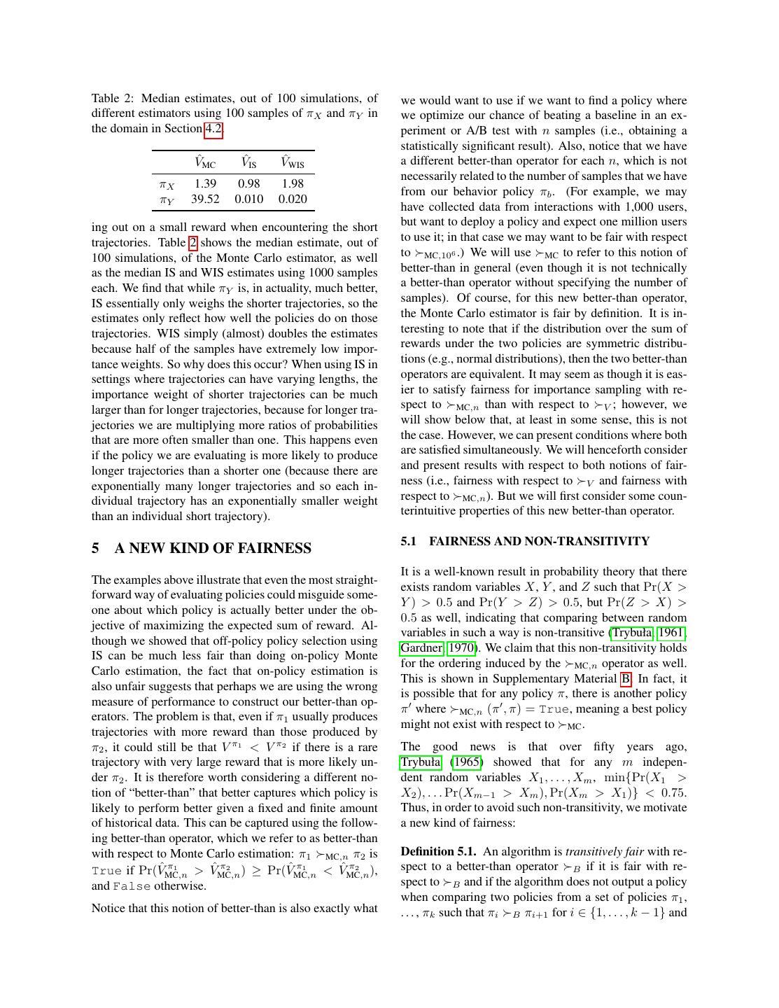
8 .1 − δMC δ for some δ ≤ 0.5, and for all k ∈ {1, 2, 3, . . . }, 1 Probability of Choosing Policy πY Algorithm 2 is a safe policy selection algorithm with re- 0.8 spect to MC,kn with probability 1 − δ when we have n On Policy samples drawn from πb . It is a transitively fair policy PHWIS-Evaluation 0.6 selection algorithm whenever δMC ≤ 0.25. PHWIS-Estimated PHWIS-Behavior 0.4 IS Note that these algorithms are analogous to statistical hy- WIS pothesis testing in that we compare the lower bound of 0.2 our estimate of the value of one policy with the upper bound of our estimate of the value of another policy. This 0 analogue is similar to how our fair policy selection algo- 0 20 40 60 80 rithms shared much in common with doing power analy- L ses for hypothesis testing. Also note that as with fairness, Figure 3: Probability of various estimators choosing πY Theorem 6.5 ensures safety with respect to both better- over πX for different values of L in the domain given in than operators, so if one uses Algorithm 2 with the inputs Section 4.2 with 1000 trajectories drawn from the uni- as described in Theorem 6.5, one does not have to deter- form random behavior policy. For each estimator, the mine which better-than operator one is using. Again, we probability of outputting πY was estimated using 100 in- find that safety with respect to MC is more difficult to dependent estimates. satisfy than safety with respect to V . We can formalize where L is the set of trajectory lengths that appear in the this with the following theorem. data and Wl is a weight for the relative importance of Theorem 6.6. There exists policies π1 , π2 , and behavior each trajectory length. policy πb for which Algorithm 2 with inputs as described in Theorem 6.4 is not a safe policy selection algorithm Notice that in the domain in Section 4.2, the length of the with respect to MC,1 with p = 0.5 when we have a sin- trajectories did not depend on the policy that was used gle sample drawn from πb . to generate them; in such cases, we can use the follow- |{τi |Ti =l}| ing weights: Wl (Behavior) n . The weights 7 PRACTICAL FAIRNESS: simply count the proportion of trajectories in our data (i.e., generated by the behavior policy) that have length VARYING TRAJECTORY LENGTHS l. We will refer to PHWIS with this weighting scheme as PHWIS-Behavior. Now we will see how this esti- While the algorithms above provide a way to guarantee mator performs on the domain in Section 4.2 (Figure 2) fairness, the concentration inequalities we used are nat- where L ∈ {1, 3, 5, 10, 20, 40, 60, 80} given 1000 trajec- urally quite loose in most cases, and would likely result tories from the uniform random behavior policy. Figure 3 in returning No Fair Comparison in many cases. shows that while IS and WIS are unfair (choose πX more Practically, it would be desirable to have algorithms that often than πY ) when the long trajectories are of length can provide fair comparisons more often. As a first step 20, PHWIS-Behavior always chooses the policy that the in this direction, here we discuss a heuristic approach to on-policy Monte Carlo estimator would choose (i.e., πX policy selection for domains where we have varying tra- when L = 1, and πY otherwise). jectory lengths, as seen in Section 4.2. The reason for fo- cusing on this particular aspect of unfairness is because However, note that in cases where different policies it is systematic (potentially arising in any domain where may generate trajectories of different lengths (for ex- trajectories vary in length), yet it seems like there should ample, bad policies causing users to dropout sooner), be a way to correct for the systematic preference towards this simple form of weighting might not work too well. shorter trajectories in practically relevant domains. The Ideally, we would like to use the following weights: idea we propose here is to compute an IS-based estimate Wl (Evaluation) Pr(1 (|τ | = l|τ ∼ πe )), where πe is for each trajectory length individually and then recom- the evaluation policy for which we would like to esti- bine the estimates to get a new estimate. We propose us- mate Vˆ πe . We cannot actually compute these weights ing the following estimator, which we refer to as the Per- because we do not know the probability of any trajec- Horizon Weighted Importance Sampling (PHWIS) esti- tory being generated by the evaluation policy, but when mator: we have ground truth, we can use the PHWIS-Evaluation estimator as a point of comparison. To approximate these Ti 1 weights, we can take the weighted importance sampling VˆPHWIS = Wl wi Ri,t estimate of the trajectory lengths generated by the be- {τi |Ti =l} wi t=1 n l∈L {τi |Ti =l} 1 havior policy: Wl (WIS) n wi i=1 wi 1 (Ti = l) i=1 WIS estimate on l-length trajectories 

9 .(i.e., rather than reweighing the rewards of all the tra- 1 Probability of Choosing Policy πY jectories generated by the behavior policy, we reweigh 0.8 the probability that trajectories of length l are gener- ated by the behavior policy). While this is a seem- 0.6 ingly reasonable thing to do, this estimate will still suffer from high variance for the same reason the 0.4 WIS estimator does, which would again lead to as- signing small weights for longer trajectories. Instead 0.2 we propose a heuristic way to make weights for dif- ferent trajectory lengths have comparable magnitudes: 0 1 n 1/Ti 1 2 3 4 5 6 Wl (Estimated) n i=1 wi 1 (Ti = l). The i=1 wi r idea behind these weights is that they should give us a sense of which weights are preferred by the evaluation Figure 4: Probability of various estimators choosing πY policy while maintaining that weights of different trajec- over πX for different values of r in the domain given in tory lengths have comparable magnitudes. As we see Section 7.1. in Figure 3, PHWIS-Estimated has almost identical per- formance to PHWIS-Behavior and PHWIS-Evaluation value of r (except for PHWIS-Behavior when r = 1). (with just a small probability of choosing the wrong pol- PHWIS-Evaluation tracks the on-policy estimator rea- icy when both trajectory lengths are short). However, the sonably well, only sometimes choosing the wrong pol- true value of using such an estimator comes in domains icy in the r = 4 case. PHWIS-Estimated similarly tracks where the length of a trajectory depends on the policy, the on-policy estimator reasonably well, but it sometimes and so PHWIS-Behavior may not be sufficient. We now chooses the wrong policy in the r = 3 case and is un- examine one such domain. fair when r = 4. Thus, PHWIS-Estimated seems to be a reasonable policy selection estimator to use in such 7.1 POLICY-DEPENDENT TRAJECTORY domains, and can be much better than using PHWIS- LENGTHS Behavior in some cases. Consider a MDP that has three states—s0 , s1 , and s2 — 8 CONCLUSION and two actions—X and Y . The agent starts in s0 and, on the first time step, if the agent takes action X, they In this paper, we examined the problem of off-policy pol- deterministically transition to s1 and receives a reward icy selection and introduced a new property for policy of r, and if the agent takes action Y , they transition de- selection algorithms called fairness. We showed that im- terministically to s2 and receive a reward of 1. Thereafter portance sampling is unfair when used for policy selec- the agent will always remain in the same state until the tion even though it is an unbiased estimator for policy trajectory ends and will receive a reward of r whenever evaluation. We presented two approaches to deal with it takes action X in state s1 , a reward of 1 whenever it this issue, a theoretical solution and a new practical es- takes action Y in state s2 , and a reward of 0 otherwise. If timator. This is but a first step in tackling the issue of the first action was X, the trajectory will end with prob- fairness in off-policy policy selection. Our hope is that ability 0.05 after each action, and if the first action was our introduction of the notion of fairness for policy se- Y , the trajectory will end with probability 0.01 after each lection will result in growing interest on the challenges action. Thus, taking action Y in the beginning will result involved in doing off-policy policy selection, including in a trajectory that is five times as long in expectation. how unfairness propagates to policy search methods that optimize over an infinite class of policies. The behavior policy πb takes each action with probabil- ity 0.5. Again, we want to compare two policies: πX , Acknowledgements which takes action X with probability 0.99, and πY , which takes action Y with probability 0.99. Whether πX The research reported here was supported, in whole or in or πY is better will depend on r. The policies have the part, by the Institute of Education Sciences, U.S. Depart- same value when r = 5, because the difference in re- ment of Education, through Grants R305A130215 and wards offsets the difference in lengths. R305B150008 to Carnegie Mellon University. The opin- Figure 4 shows which policy is chosen when using dif- ions expressed are those of the authors and do not rep- ferent estimators for the domain described above with resent views of the Institute or the U.S. Dept. of Educa- various values for r. We find that the IS, WIS, and even tion. The research was also supported in part by a NSF PHWIS-Behavior estimators are unfair regardless of the CAREER grant. 

10 .References S. Trybuła. On the paradox of n random variables. Ap- plicationes Mathematicae, 8(2):143–156, 1965. M. Dud´ık, J. Langford, and L. Li. Doubly robust policy Z. Wang, V. Bapst, N. Heess, V. Mnih, R. Munos, evaluation and learning. In International Conference K. Kavukcuoglu, and N. de Freitas. Sample efficient on Machine Learning, pages 1097–1104. Omnipress, actor-critic with experience replay. arXiv preprint 2011. arXiv:1611.01224, 2016. M. Gardner. Paradox of nontransitive dice and elusive principle of indifference. Scientific American, 223(6): 110, 1970. S. Jabbari, M. Joseph, M. Kearns, J. Morgenstern, and A. Roth. Fairness in reinforcement learning. In Inter- national Conference on Machine Learning, 2017. N. Jiang and L. Li. Doubly robust off-policy value eval- uation for reinforcement learning. In International Conference on Machine Learning, pages 652–661, 2016. T. Jie and P. Abbeel. On a connection between impor- tance sampling and the likelihood ratio policy gradi- ent. In Advances in Neural Information Processing Systems, pages 1000–1008, 2010. S. Levine and V. Koltun. Guided policy search. In Inter- national Conference on Machine Learning, pages 1–9, 2013. T. Mandel, Y.-E. Liu, S. Levine, E. Brunskill, and Z. Popovic. Offline policy evaluation across repre- sentations with applications to educational games. In Internatonal Conference on Autonomous Agents and Multi-Agent Systems, pages 1077–1084. International Foundation for Autonomous Agents and Multiagent Systems, 2014. M. Powell and J. Swann. Weighted uniform sampling—a Monte Carlo technique for reducing variance. IMA Journal of Applied Mathematics, 2(3):228–236, 1966. D. Precup, R. S. Sutton, and S. Singh. Eligibility traces for off-policy policy evaluation. In International Con- ference on Machine Learning. Citeseer, 2000. P. S. Thomas and E. Brunskill. Data-efficient off-policy policy evaluation for reinforcement learning. In In- ternational Conference on Machine Learning, pages 2139–2148, 2016. P. S. Thomas and E. Brunskill. Importance sampling with unequal support. In AAAI, pages 2646–2652, 2017. P. S. Thomas, G. Theocharous, and M. Ghavamzadeh. High-confidence off-policy evaluation. In AAAI, pages 3000–3006, 2015a. P. S. Thomas, G. Theocharous, and M. Ghavamzadeh. High confidence policy improvement. In International Conference on Machine Learning, 2015b. S. Trybuła. On the paradox of three random variables. Applicationes Mathematicae, 4(5):321–332, 1961. 

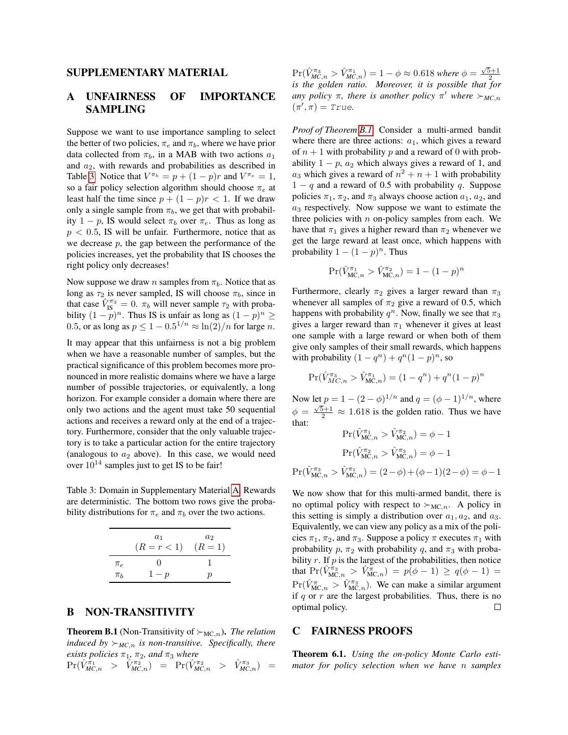
11 . √ SUPPLEMENTARY MATERIAL Pr(VˆMC,n π3 > VˆMC,n π1 ) = 1 − φ ≈ 0.618 where φ = 5+1 2 is the golden ratio. Moreover, it is possible that for A UNFAIRNESS OF IMPORTANCE any policy π, there is another policy π where MC,n SAMPLING (π , π) = True. Suppose we want to use importance sampling to select Proof of Theorem B.1. Consider a multi-armed bandit the better of two policies, πe and πb , where we have prior where there are three actions: a1 , which gives a reward data collected from πb , in a MAB with two actions a1 of n + 1 with probability p and a reward of 0 with prob- and a2 , with rewards and probabilities as described in ability 1 − p, a2 which always gives a reward of 1, and Table 3. Notice that V πb = p + (1 − p)r and V πe = 1, a3 which gives a reward of n2 + n + 1 with probability so a fair policy selection algorithm should choose πe at 1 − q and a reward of 0.5 with probability q. Suppose least half the time since p + (1 − p)r < 1. If we draw policies π1 , π2 , and π3 always choose action a1 , a2 , and only a single sample from πb , we get that with probabil- a3 respectively. Now suppose we want to estimate the ity 1 − p, IS would select πb over πe . Thus as long as three policies with n on-policy samples from each. We p < 0.5, IS will be unfair. Furthermore, notice that as have that π1 gives a higher reward than π2 whenever we we decrease p, the gap between the performance of the get the large reward at least once, which happens with policies increases, yet the probability that IS chooses the probability 1 − (1 − p)n . Thus right policy only decreases! Pr(VˆMC,n π1 > VˆMC,n π2 ) = 1 − (1 − p)n Now suppose we draw n samples from πb . Notice that as long as τ2 is never sampled, IS will choose πb , since in Furthermore, clearly π2 gives a larger reward than π3 that case VˆISπ3 = 0. πb will never sample τ2 with proba- whenever all samples of π2 give a reward of 0.5, which bility (1 − p)n . Thus IS is unfair as long as (1 − p)n ≥ happens with probability q n . Now, finally we see that π3 0.5, or as long as p ≤ 1 − 0.51/n ≈ ln(2)/n for large n. gives a larger reward than π1 whenever it gives at least one sample with a large reward or when both of them It may appear that this unfairness is not a big problem give only samples of their small rewards, which happens when we have a reasonable number of samples, but the with probability (1 − q n ) + q n (1 − p)n , so practical significance of this problem becomes more pro- nounced in more realistic domains where we have a large Pr(VˆM π3 ˆ π1 n n C,n > VMC,n ) = (1 − q ) + q (1 − p) n number of possible trajectories, or equivalently, a long horizon. For example consider a domain where there are Now let √ p = 1 − (2 − φ)1/n and q = (φ − 1)1/n , where only two actions and the agent must take 50 sequential 5+1 φ = 2 ≈ 1.618 is the golden ratio. Thus we have actions and receives a reward only at the end of a trajec- that: tory. Furthermore, consider that the only valuable trajec- Pr(VˆMC,n π1 > VˆMC,n π2 )=φ−1 tory is to take a particular action for the entire trajectory (analogous to a2 above). In this case, we would need Pr(VˆMC,n π2 > VˆMC,n π3 )=φ−1 over 1014 samples just to get IS to be fair! Pr(VˆMC,n π3 > VˆMC,n π1 ) = (2 − φ) + (φ − 1)(2 − φ) = φ − 1 Table 3: Domain in Supplementary Material A. Rewards We now show that for this multi-armed bandit, there is are deterministic. The bottom two rows give the proba- no optimal policy with respect to MC,n . A policy in bility distributions for πe and πb over the two actions. this setting is simply a distribution over a1 , a2 , and a3 . Equivalently, we can view any policy as a mix of the poli- a1 a2 cies π1 , π2 , and π3 . Suppose a policy π executes π1 with (R = r < 1) (R = 1) probability p, π2 with probability q, and π3 with proba- πe 0 1 bility r. If p is the largest of the probabilities, then notice πb 1−p p that Pr(VˆMC,n π3 > VˆMC,n π ) = p(φ − 1) ≥ q(φ − 1) = ˆ π ˆ π3 Pr(VMC,n > VMC,n ). We can make a similar argument if q or r are the largest probabilities. Thus, there is no optimal policy. B NON-TRANSITIVITY Theorem B.1 (Non-Transitivity of MC,n ). The relation C FAIRNESS PROOFS induced by MC,n is non-transitive. Specifically, there exists policies π1 , π2 , and π3 where Theorem 6.1. Using the on-policy Monte Carlo esti- Pr(VˆMC,n π1 > VˆMC,n π2 ) = Pr(VˆMC,n π2 > VˆMC,n π3 ) = mator for policy selection when we have n samples 

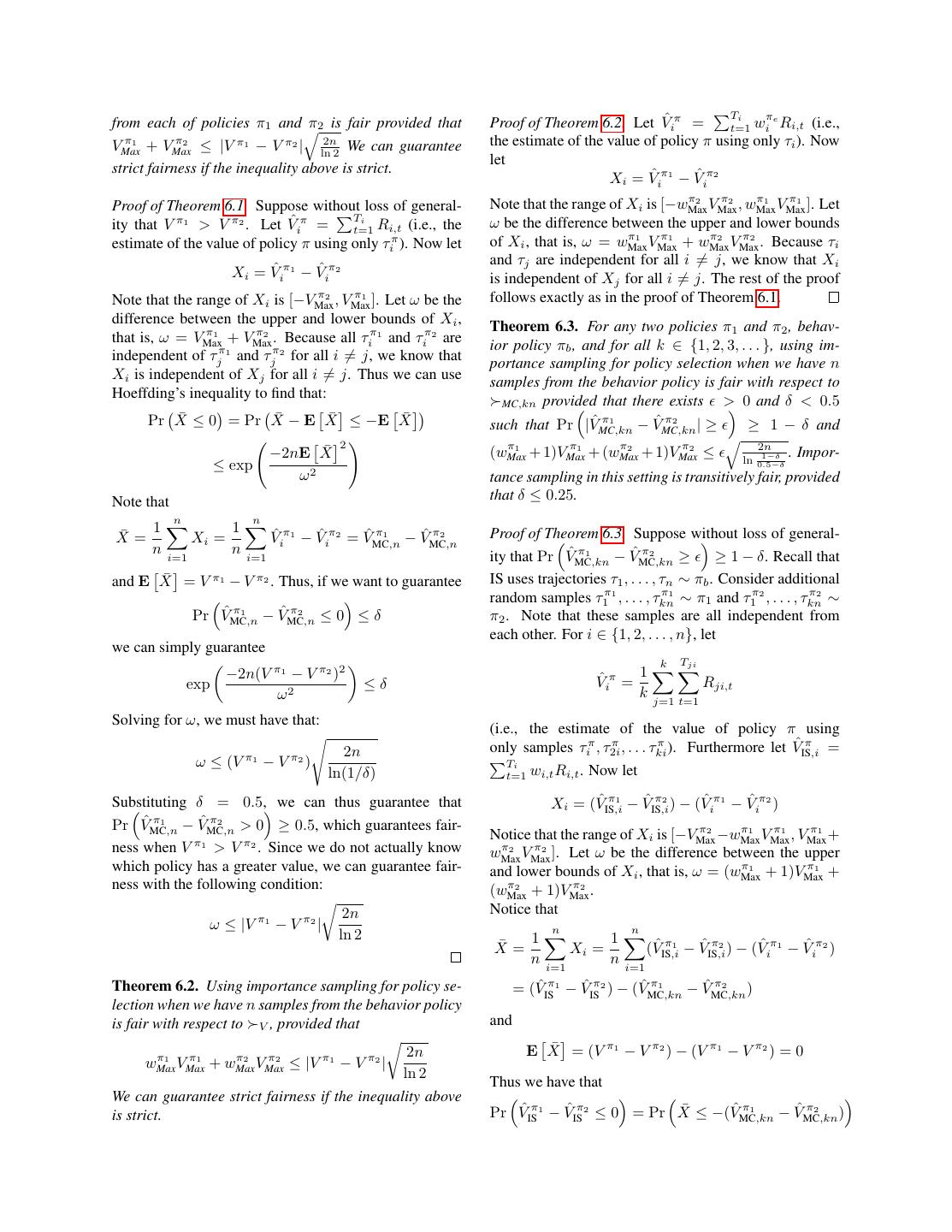
12 . Ti from each of policies π1 and π2 is fair provided that Proof of Theorem 6.2. Let Vˆiπ = πe t=1 wi Ri,t (i.e., π1 VMax π2 + VMax ≤ |V π1 − V π2 | ln 2n the estimate of the value of policy π using only τi ). Now 2 We can guarantee let strict fairness if the inequality above is strict. Xi = Vˆiπ1 − Vˆiπ2 π2 π2 π1 π1 Proof of Theorem 6.1. Suppose without loss of general- Note that the range of Xi is [−wMax VMax , wMax VMax ]. Let Ti ity that V π1 > V π2 . Let Vˆiπ = t=1 Ri,t (i.e., the ω be the difference between the upper and lower bounds π1 π1 π2 π2 estimate of the value of policy π using only τiπ ). Now let of Xi , that is, ω = wMax VMax + wMax VMax . Because τi and τj are independent for all i = j, we know that Xi Xi = Vˆiπ1 − Vˆiπ2 is independent of Xj for all i = j. The rest of the proof π2 π1 follows exactly as in the proof of Theorem 6.1. Note that the range of Xi is [−VMax , VMax ]. Let ω be the difference between the upper and lower bounds of Xi , Theorem 6.3. For any two policies π1 and π2 , behav- π1 π2 that is, ω = VMax + VMax . Because all τiπ1 and τiπ2 are ior policy πb , and for all k ∈ {1, 2, 3, . . . }, using im- π1 π2 independent of τj and τj for all i = j, we know that portance sampling for policy selection when we have n Xi is independent of Xj for all i = j. Thus we can use samples from the behavior policy is fair with respect to Hoeffding’s inequality to find that: > 0 and δ < 0.5 MC,kn provided that there exists ¯ ≤ 0 = Pr X Pr X ¯ −E X ¯ ≤ −E X ¯ such that Pr |V ˆ π1 −V ˆ π2 |≥ ≥ 1 − δ and MC,kn MC,kn 2 π1 π1 π2 π2 2n −2nE X ¯ (wMax + 1)VMax + (wMax + 1)VMax ≤ 1−δ . Impor- ln ≤ exp 2 0.5−δ ω tance sampling in this setting is transitively fair, provided Note that that δ ≤ 0.25. n n ¯= 1 X Xi = 1 Vˆiπ1 − Vˆiπ2 = VˆMC,n π1 − VˆMC,n π2 Proof of Theorem 6.3. Suppose without loss of general- n n i=1 i=1 ity that Pr VˆMC,kn π1 − VˆMC,kn π2 ≥ ≥ 1 − δ. Recall that ¯ = V π1 − V π2 . Thus, if we want to guarantee and E X IS uses trajectories τ1 , . . . , τn ∼ πb . Consider additional random samples τ1π1 , . . . , τkn π1 ∼ π1 and τ1π2 , . . . , τkn π2 ∼ Pr VˆMC,n π1 − VˆMC,n π2 ≤0 ≤δ π2 . Note that these samples are all independent from each other. For i ∈ {1, 2, . . . , n}, let we can simply guarantee k Tji −2n(V π1 − V π2 )2 1 exp ≤δ Vˆiπ = Rji,t ω2 k j=1 t=1 Solving for ω, we must have that: (i.e., the estimate of the value of policy π using 2n only samples τiπ , τ2i π π , . . . τki ). Furthermore let VˆIS,i π = ω ≤ (V π1 − V π2 ) Ti ln(1/δ) t=1 wi,t Ri,t . Now let Substituting δ = 0.5, we can thus guarantee that Xi = (VˆIS,i π1 − VˆIS,i π2 ) − (Vˆiπ1 − Vˆiπ2 ) Pr VˆMC,n π1 − VˆMC,n π2 > 0 ≥ 0.5, which guarantees fair- π2 π1 π1 π1 Notice that the range of Xi is [−VMax −wMax VMax , VMax + ness when V π1 > V π2 . Since we do not actually know π2 π2 wMax VMax ]. Let ω be the difference between the upper which policy has a greater value, we can guarantee fair- π1 and lower bounds of Xi , that is, ω = (wMax + 1)VMaxπ1 + ness with the following condition: π2 π2 (wMax + 1)VMax . 2n Notice that ω ≤ |V π1 − V π2 | n n ln 2 ¯= 1 X Xi = 1 (VˆIS,i π1 − VˆIS,i π2 ) − (Vˆiπ1 − Vˆiπ2 ) n i=1 n i=1 Theorem 6.2. Using importance sampling for policy se- = (VˆISπ1 − VˆISπ2 ) − (VˆMC,kn π1 − VˆMC,kn π2 ) lection when we have n samples from the behavior policy is fair with respect to V , provided that and 2n ¯ = (V π1 − V π2 ) − (V π1 − V π2 ) = 0 E X π1 π1 π2 π2 wMax VMax + wMax VMax ≤ |V π1 − V π2 | ln 2 Thus we have that We can guarantee strict fairness if the inequality above is strict. Pr VˆISπ1 − VˆISπ2 ≤ 0 = Pr X ¯ ≤ −(Vˆ π1 ˆ π2 MC,kn − VMC,kn ) 

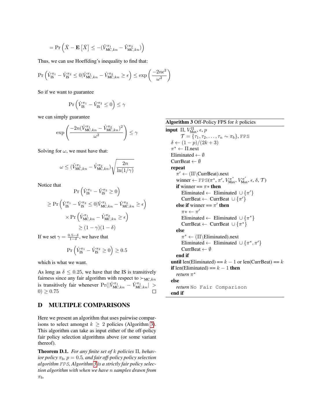
13 . ¯ −E X ¯ ≤ −(Vˆ π1 ˆ π2 = Pr X MC,kn − VMC,kn ) Thus, we can use Hoeffding’s inequality to find that: 2 −2n Pr VˆISπ1 − VˆISπ2 ≤ 0|VˆMC,kn π1 − VˆMC,kn π2 ≥ ≤ exp ω2 So if we want to guarantee Pr VˆISπ1 − VˆISπ2 ≤ 0 ≤ γ we can simply guarantee Algorithm 3 Off-Policy FPS for k policies −2n(VˆMC,kn π1 − VˆMC,kn π2 )2 input Π, VMax Π , ,p exp ≤γ ω2 T = {τ1 , τ2 , . . . , τn ∼ πb }, FPS δ ← (1 − p)/(2k + 3) Solving for ω, we must have that: π ∗ ← Π.next Eliminated ← ∅ 2n CurrBeat ← ∅ ω ≤ (VˆMC,kn π1 − VˆMC,kn π2 ) repeat ln(1/γ) π ← (Π\CurrBeat).next π∗ winner ← FPS(π ∗ , π , VMax π , VMax , , δ, T ) Notice that if winner == π∗ then Pr VˆISπ1 − VˆISπ2 ≥ 0 Eliminated ← Eliminated ∪ {π } CurrBeat ← CurrBeat ∪ {π } ≥ Pr VˆISπ1 − VˆISπ2 ≤ 0|VˆMC,kn π1 − VˆMC,kn π2 ≥ else if winner == π then π∗ ← π × Pr VˆMC,kn π1 − VˆMC,kn π2 ≥ Eliminated ← Eliminated ∪ {π ∗ } CurrBeat ← CurrBeat ∪ {π ∗ } ≥ (1 − γ)(1 − δ) else If we set γ = 0.5−δ 1−δ , we have that π ∗ ← (Π\Eliminated).next Eliminated ← Eliminated ∪ {π ∗ , π } Pr VˆISπ1 − VˆISπ2 ≥ 0 ≥ 0.5 CurrBeat ← ∅ end if which is what we want. until len(Eliminated) == k − 1 or len(CurrBeat) == k if len(Eliminated) == k − 1 then As long as δ ≤ 0.25, we have that the IS is transitively return π ∗ fairness since any fair algorithm with respect to MC,kn else is transitively fair whenever Pr(|VˆMC,kn π1 − VˆMC,kn π1 | > return No Fair Comparison 0) ≥ 0.75 end if D MULTIPLE COMPARISONS Here we present an algorithm that uses pairwise compar- isons to select amongst k ≥ 2 policies (Algorithm 3). This algorithm can take as input either of the off-policy fair policy selection algorithms above (or some variant thereof). Theorem D.1. For any finite set of k policies Π, behav- ior policy πb , p = 0.5, and fair off-policy policy selection algorithm FPS, Algorithm 3 is a strictly fair policy selec- tion algorithm with when we have n samples drawn from πb . 

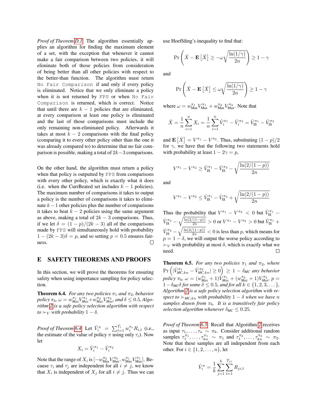
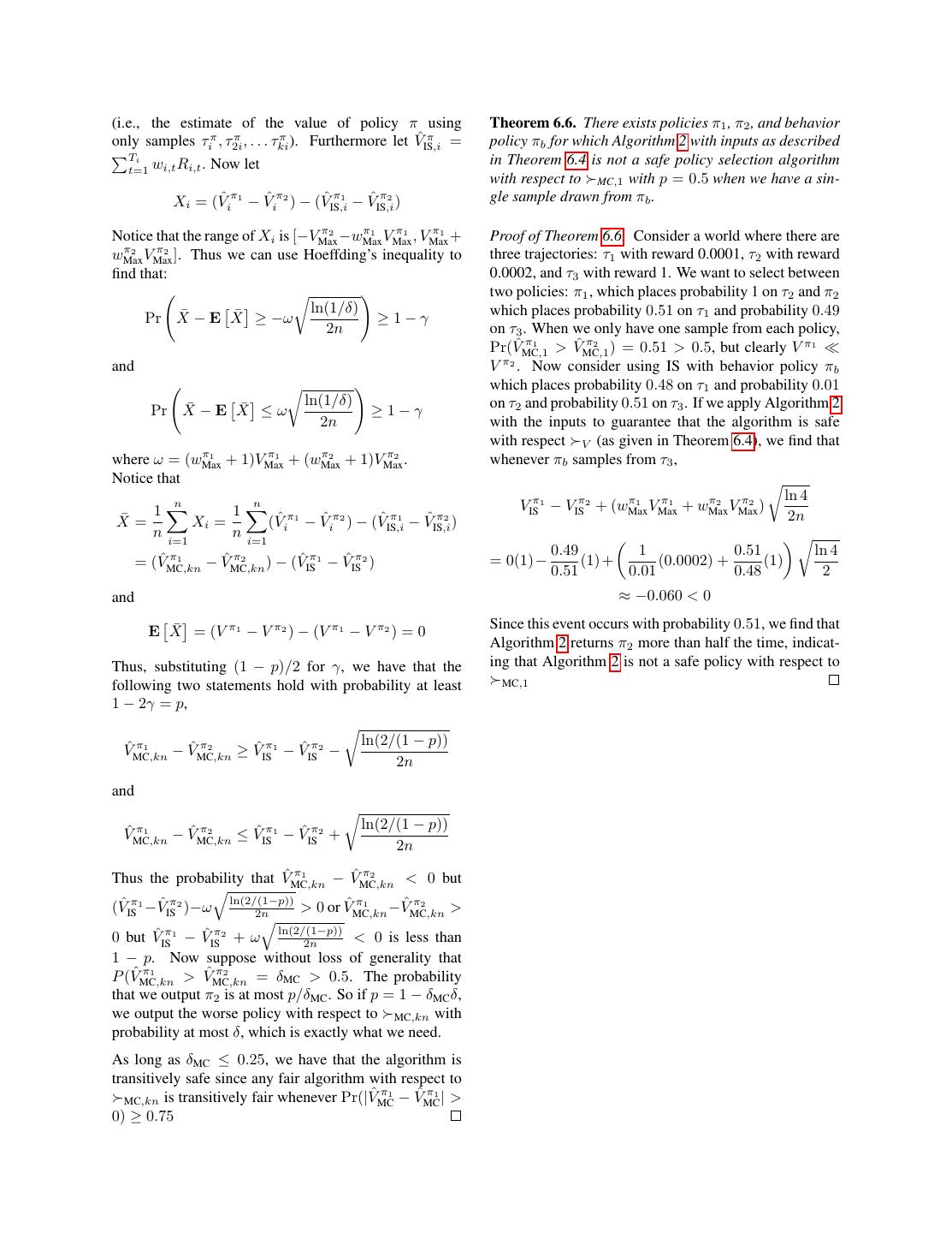
14 .Proof of Theorem D.1. The algorithm essentially ap- use Hoeffding’s inequality to find that: plies an algorithm for finding the maximum element of a set, with the exception that whenever it cannot ln(1/γ) ¯ −E X Pr X ¯ ≥ −ω ≥1−γ make a fair comparison between two policies, it will 2n eliminate both of those policies from consideration of being better than all other policies with respect to and the better-than function. The algorithm must return No Fair Comparison if and only if every policy ln(1/γ) is eliminated. Notice that we only eliminate a policy ¯ −E X Pr X ¯ ≤ω ≥1−γ 2n when it is not returned by FPS or when No Fair Comparison is returned, which is correct. Notice π1 π1 π2 π2 where ω = wMax VMax + wMax VMax . Note that that until there are k − 1 policies that are eliminated, at every comparison at least one policy is eliminated n n and the last of those comparisons must include the ¯= 1 X Xi = 1 Vˆiπ1 − Vˆiπ2 = VˆISπ1 − VˆISπ2 only remaining non-eliminated policy. Afterwards it n i=1 n i=1 takes at most k − 2 comparisons with the final policy (comparing it to every other policy other than the one it and E X ¯ = V π1 − V π2 . Thus, substituting (1 − p)/2 was already compared to) to determine that no fair com- for γ, we have that the following two statements hold parison is possible, making a total of 2k−3 comparisons. with probability at least 1 − 2γ = p, ln(2/(1 − p)) On the other hand, the algorithm must return a policy V π1 − V π2 ≥ VˆISπ1 − VˆISπ2 − when that policy is outputted by FPS from comparisons 2n with every other policy, which is exactly what it does and (i.e. when the CurrBeated set includes k − 1 policies). The maximum number of comparisons it takes to output ln(2/(1 − p)) a policy is the number of comparisons it takes to elimi- V π1 − V π2 ≤ VˆISπ1 − VˆISπ2 + 2n nate k − 1 other policies plus the number of comparisons it takes to beat k − 2 policies using the same argument Thus the probability that V π1 − V π2 < 0 but VˆISπ1 − as above, making a total of 2k − 3 comparisons. Thus, if we let δ = (1 − p)/(2k − 3) all of the comparisons VˆISπ2 − ln(2/(1−p)) 2n > 0 or V π1 − V π2 > 0 but VˆISπ1 + made by FPS will simultaneously hold with probability VˆISπ2 − ln(2/(1−p)) < 0 is less than p, which means for 2n 1 − (2k − 3)δ = p, and so setting p = 0.5 ensures fair- p = 1 − δ, we will output the worse policy according to ness. V with probability at most δ, which is exactly what we need. E SAFETY THEOREMS AND PROOFS Theorem 6.5. For any two policies π1 and π2 , where In this section, we will prove the theorems for ensuring Pr |VˆMC,kn π1 − VˆMC,kn π2 | ≥ 0 ≥ 1 − δMC any behavior π1 π1 π2 π2 safety when using importance sampling for policy selec- policy πb , ω = (wMax + 1)VMax + (wMax + 1)VMax ,p= tion. 1 − δMC δ for some δ ≤ 0.5, and for all k ∈ {1, 2, 3, . . . }, Algorithm 2 is a safe policy selection algorithm with re- Theorem 6.4. For any two policies π1 and π2 , behavior π1 π1 π2 π2 spect to MC,kn with probability 1 − δ when we have n policy πb , ω = wMax VMax +wMax VMax , and δ ≤ 0.5, Algo- samples drawn from πb . It is a transitively fair policy rithm 2 is a safe policy selection algorithm with respect selection algorithm whenever δMC ≤ 0.25. to V with probability 1 − δ. Ti Proof of Theorem 6.5. Recall that Algorithm 2 receives Proof of Theorem 6.4. Let Vˆiπ = πe t=1 wi Ri,t (i.e., as input τ1 , . . . , τn ∼ πb . Consider additional random the estimate of the value of policy π using only τi ). Now samples τ1π1 , . . . , τkn π1 ∼ π1 and τ1π2 , . . . , τkn π2 ∼ π2 . let Note that these samples are all independent from each Xi = Vˆ π1 − Vˆ π2 i i other. For i ∈ {1, 2, . . . , n}, let π2 π2 π1 π1 Note that the range of Xi is [−wMax VMax , wMax VMax ]. Be- k Tji cause τi and τj are independent for all i = j, we know 1 Vˆiπ = Rji,t that Xi is independent of Xj for all i = j. Thus we can k j=1 t=1 

15 .(i.e., the estimate of the value of policy π using Theorem 6.6. There exists policies π1 , π2 , and behavior only samples τiπ , τ2i π π , . . . τki ). Furthermore let VˆIS,i π = policy πb for which Algorithm 2 with inputs as described Ti in Theorem 6.4 is not a safe policy selection algorithm t=1 wi,t Ri,t . Now let with respect to MC,1 with p = 0.5 when we have a sin- Xi = (Vˆiπ1 − Vˆiπ2 ) − (VˆIS,i π1 − VˆIS,i π2 ) gle sample drawn from πb . π2 π1 π1 π1 Notice that the range of Xi is [−VMax −wMax VMax , VMax + Proof of Theorem 6.6. Consider a world where there are π2 π2 wMax VMax ]. Thus we can use Hoeffding’s inequality to three trajectories: τ1 with reward 0.0001, τ2 with reward find that: 0.0002, and τ3 with reward 1. We want to select between two policies: π1 , which places probability 1 on τ2 and π2 ¯ −E X ¯ ≥ −ω ln(1/δ) which places probability 0.51 on τ1 and probability 0.49 Pr X ≥1−γ 2n on τ3 . When we only have one sample from each policy, Pr(VˆMC,1 π1 > VˆMC,1 π2 ) = 0.51 > 0.5, but clearly V π1 π2 and V . Now consider using IS with behavior policy πb which places probability 0.48 on τ1 and probability 0.01 ¯ −E X ¯ ≤ω ln(1/δ) on τ2 and probability 0.51 on τ3 . If we apply Algorithm 2 Pr X ≥1−γ 2n with the inputs to guarantee that the algorithm is safe with respect V (as given in Theorem 6.4), we find that π1 π1 π2 π2 where ω = (wMax + 1)VMax + (wMax + 1)VMax . whenever πb samples from τ3 , Notice that ln 4 n n VISπ1 − VISπ2 + (wMax π1 π1 VMax π2 + wMax π2 VMax ) ¯= 1 X Xi = 1 (Vˆiπ1 − Vˆiπ2 ) − (VˆIS,i π1 − VˆIS,i π2 ) 2n n i=1 n i=1 0.49 1 0.51 ln 4 = (VˆMC,kn π1 − VˆMC,kn π2 ) − (VˆISπ1 − VˆISπ2 ) = 0(1) − (1) + (0.0002) + (1) 0.51 0.01 0.48 2 and ≈ −0.060 < 0 ¯ = (V π1 − V π2 ) − (V π1 − V π2 ) = 0 Since this event occurs with probability 0.51, we find that E X Algorithm 2 returns π2 more than half the time, indicat- Thus, substituting (1 − p)/2 for γ, we have that the ing that Algorithm 2 is not a safe policy with respect to following two statements hold with probability at least MC,1 1 − 2γ = p, ln(2/(1 − p)) VˆMC,kn π1 − VˆMC,kn π2 ≥ VˆISπ1 − VˆISπ2 − 2n and ln(2/(1 − p)) VˆMC,kn π1 − VˆMC,kn π2 ≤ VˆISπ1 − VˆISπ2 + 2n Thus the probability that VˆMC,kn π1 − VˆMC,kn π2 < 0 but ln(2/(1−p)) (VˆISπ1 −VˆISπ2 )−ω 2n > 0 or VˆMC,kn π1 −VˆMC,kn π2 > 0 but VˆISπ1 − VˆISπ2 + ω ln(2/(1−p)) 2n < 0 is less than 1 − p. Now suppose without loss of generality that P (VˆMC,kn π1 > VˆMC,kn π2 = δMC > 0.5. The probability that we output π2 is at most p/δMC . So if p = 1 − δMC δ, we output the worse policy with respect to MC,kn with probability at most δ, which is exactly what we need. As long as δMC ≤ 0.25, we have that the algorithm is transitively safe since any fair algorithm with respect to ˆ π1 ˆ π1 MC,kn is transitively fair whenever Pr(|VMC − VMC | > 0) ≥ 0.75