A Hitting Time Analysis of Stoch

1 . A Hitting Time Analysis of Stochastic Gradient Langevin Dynamics Yuchen Zhang∗ Percy Liang† Moses Charikar‡ April 10, 2018 arXiv:1702.05575v3 [cs.LG] 9 Apr 2018 Abstract We study the Stochastic Gradient Langevin Dynamics (SGLD) algorithm for non-convex optimization. The algorithm performs stochastic gradient descent, where in each step it injects appropriately scaled Gaussian noise to the update. We analyze the algorithm’s hitting time to an arbitrary subset of the parameter space. Two results follow from our general theory: First, we prove that for empirical risk minimization, if the empirical risk is pointwise close to the (smooth) population risk, then the algorithm finds an approximate local minimum of the population risk in polynomial time, escaping suboptimal local minima that only exist in the empirical risk. Second, we show that SGLD improves on one of the best known learnability results for learning linear classifiers under the zero-one loss. 1 Introduction A central challenge of non-convex optimization is avoiding sub-optimal local minima. Although escaping all local minima is NP-hard in general [e.g. 7], one might expect that it should be possible to escape “ap- propriately shallow” local minima, whose basins of attraction have relatively low barriers. As an illustrative example, consider minimizing an empirical risk function in Figure 1. As the figure shows, although the empirical risk is uniformly close to the population risk, it contains many poor local minima that don’t exist in the population risk. Gradient descent is unable to escape such local minima. A natural workaround is to inject random noise to the gradient. Empirically, adding gradient noise has been found to improve learning for deep neural networks and other non-convex models [23, 24, 18, 17, 35]. However, theoretical understanding of the value of gradient noise is still incomplete. For example, Ge et al. [14] show that by adding isotropic noise w and by choosing a sufficiently small stepsize η, the iterative update: x ← x − η (∇f (x) + w) (1) is able to escape strict saddle points. Unfortunately, this approach, as well as the subsequent line of work on escaping saddle points [20, 2, 1], doesn’t guarantee escaping even shallow local minima. Another line of work in Bayesian statistics studies the Langevin Monte Carlo (LMC) method [28], which employs an alternative noise term. Given a function f , LMC performs the iterative update: x ← x − η (∇f (x) + 2/(ηξ) w) where w ∼ N (0, I), (2) ∗ Computer Science Department, Stanford University, Stanford, CA 94305. Email: zhangyuc@cs.stanford.edu. † Computer Science Department, Stanford University, Stanford, CA 94305. Email: pliang@cs.stanford.edu. ‡ Computer Science Department, Stanford University, Stanford, CA 94305. Email: moses@cs.stanford.edu. 1 

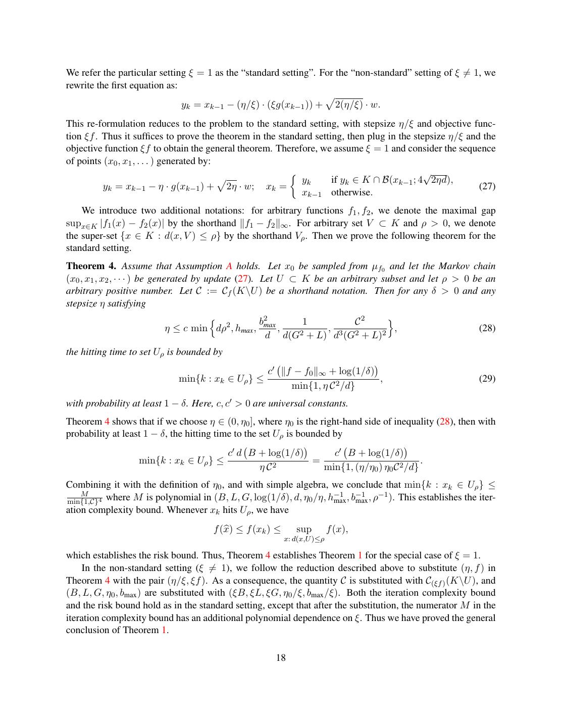
2 . 0.92 Empirical risk 0.90 Population risk 0.88 function value 0.86 0.84 0.82 3 2 1 0 1 2 3 x value Figure 1: Empirical risk (sample size = 5000) versus population risk (sample size → ∞) on one-dimensional zero- one losses. The two functions are uniformly close, but the empirical risk contains local minima that that are far worse than the population local minima. where ξ > 0 is a “temperature” hyperparameter. Unlike the bounded noise added in formula (1), LMC adds a large noise term that scales with 1/η. With a small enough η, the noise dominates the gradient, enabling the algorithm to escape any local minimum. For empirical risk minimization, one might substitute the exact gradient ∇f (x) with a stochastic gradient, which gives the Stochastic Gradient Langevin Dynamics (SGLD) algorithm [34]. It can be shown that both LMC and SGLD asymptotically converge to a stationary distribution µ(x) ∝ e−ξf (x) [28, 30]. As ξ → ∞, the probability mass of µ concentrates on the global minimum of the function f , and the algorithm asymptotically converges to a neighborhood of the global minimum. Despite asymptotic consistency, there is no theoretical guarantee that LMC is able to find the global minimum of a general non-convex function, or even a local minimum of it, in polynomial time. Recent works focus on bounding the mixing time (i.e. the time for converging to µ) of LMC and SGLD. Bubeck et al. [10], Dalalyan [12] and Bonis [8] prove that on convex functions, LMC converges to the stationary distribution in polynomial time. On non-convex functions, however, an exponentially long mixing time is unavoidable in general. According to Bovier et al. [9], it takes the Langevin diffusion at least eΩ(ξh) time to escape a depth-h basin of attraction. Thus, if the function contains multiple “deep” basins with h = Ω(1), then the mixing time is lower bounded by eΩ(ξ) . In parallel work to this paper, Raginsky et al. [27] upper bound the time of SGLD converging to an approximate global minimum of non-convex functions. They show that the upper bound is polynomial in the inverse of a quantity they call the uniform spectral gap. Similar to the mixing time bound, in the presence of multiple local minima, the convergence time to an approximate global minimum can be exponential in dimension d and the temperature parameter ξ. Contributions In this paper, we present an alternative analysis of SGLD algorithm.1 Instead of bound- ing its mixing time, we bound the algorithm’s hitting time to an arbitrary set U on a general non-convex function. The hitting time captures the algorithm’s optimization efficiency, and more importantly, it enjoys polynomial rates for hitting appropriately chosen sets regardless of the mixing time, which could be expo- nential. We highlight two consequences of the generic bound: First, under suitable conditions, SGLD hits 1 The theory holds for the standard LMC algorithm as well. 2 

3 .an approximate local minimum of f , with a hitting time that is polynomial in dimension d and all hyperpa- rameters; this extends the polynomial-time guarantees proved for convex functions [10, 12, 8]. Second, the time complexity bound is stable, in the sense that any O(1/ξ) perturbation in ∞ -norm of the function f doesn’t significantly change the hitting time. This second property is the main strength of SGLD: For any function f , if there exists another function F such that f − F ∞ = O(1/ξ), then we define the set U to be the approximate local minima of F . The two properties together imply that even if we execute SGLD on function f , it hits an approximate local minimum of F in polynomial time. In other words, SGLD is able to escape “shallow” local minima of f that can be eliminated by slightly perturbing the function. This stability property is useful in studying empirical risk minimization (ERM) in situations where the empirical risk f is pointwise close to the population risk F , but has poor local minima that don’t exist in the population risk. This phenomenon has been observed in statistical estimation with non-convex penalty functions [33, 21], as well as in minimizing the zero-one loss (see Figure 1). Under this setting, our result implies that SGLD achieves an approximate local minimum of the (smooth) population risk in polynomial time, ruling out local minima that only exist in the empirical risk. It improves over recent results on non- convex optimization [14, 20, 2, 1], which compute approximate local minima only for the empirical risk. As a concrete application, we prove a stronger learnability result for the problem of learning linear clas- sifiers under the zero-one loss [3], which involves non-convex and non-smooth empirical risk minimization. Our result improves over the recent result of Awasthi et al. [4]: the method of Awasthi et al. [4] handles noisy data corrupted by a very small Massart noise (at most 1.8 × 10−6 ), while our algorithm handles Massart noise up to any constant less than 0.5. As a Massart noise of 0.5 represents completely random observations, we see that SGLD is capable of learning from very noisy data. Techniques The key step of our analysis is to define a positive quantity called the restricted Cheeger con- stant. This quantity connects the hitting time of SGLD, the geometric properties of the objective function, and the stability of the time complexity bound. For an arbitrary function f : K → R and an arbitrary set V ⊂ K, the restricted Cheeger constant is defined as the minimal ratio between the surface area of a subset A ⊂ V and its volume with respect to a measure µ(x) ∝ e−f (x) . We prove that the hitting time is poly- nomial in the inverse of the restricted Cheeger constant (Section 2.3). The stability of the time complexity bound follows as a natural consequence of the definition of this quantity (Section 2.2). We then develop techniques to lower bound the restricted Cheeger constant based on geometric properties of the objective function (Section 2.4). Notation For any positive integer n, we use [n] as a shorthand for the discrete set {1, 2, . . . , n}. For a rectangular matrix A, let A ∗ be its nuclear norm (i.e., the sum of singular values), and A 2 be its spectral norm (i.e., the maximal singular value). For any point x ∈ Rd and an arbitrary set V ⊂ Rd , we denote their Euclidean distance by d(x, V ) := inf y∈V x − y 2 . We use B(x; r) to denote the Euclidean ball of radius r that centers at point x. 2 Algorithm and main results In this section, we define the algorithm and the basic concepts, then present the main theoretical results of this paper. 3 

4 .Algorithm 1 Stochastic Gradient Langevin Dynamics Input: Objective function f : K → R; hyperparameters (ξ, η, kmax , D). 1. Initialize x0 ∈ K by uniformly sampling from the parameter space K. 2. For each k ∈ {1, 2, . . . , kmax }: Sample w ∼ N (0, Id×d ). Compute a stochastic gradient g(xk−1 ) such that E[g(xk−1 )|xk−1 ] = ∇f (xk−1 ). Then update: yk = xk−1 − η g(xk−1 ) + 2η/ξ w; (3a) yk if yk ∈ K ∩ B(xk−1 ; D), xk = (3b) xk−1 otherwise. Output: x = xk∗ where k ∗ := argmink {f (xk )}. 2.1 The SGLD algorithm Our goal is to minimize a function f in a compact parameter space K ⊂ Rd . The SGLD algorithm [34] is summarized in Algorithm 1. In step (3a), the algorithm performs SGD on the function f , then adds Gaussian noise to the update. Step (3b) ensures that the vector xk always belong to the parameter space, and is not too far from xk−1 of the previous iteration.2 After kmax iterations, the algorithm returns a vector x. Although standard SGLD returns the last iteration’s output, we study a variant of the algorithm which returns the best vector across all iterations. This choice is important for our analysis of hitting time. We note that evaluating f (xk ) can be computationally more expensive than computing the stochastic gradient gk , because the objective function is defined on the entire dataset, while the stochastic gradient can be computed via a single instance. Returning the best xk merely facilitates theoretical analysis and might not be necessary in practice. Because of the noisy update, the sequence (x0 , x1 , x2 , . . . ) asymptotically converges to a stationary distribution rather than a stationary point [30]. Although this fact introduces challenges to the analysis, we show that its non-asymptotic efficiency can be characterized by a positive quantity called the restricted Cheeger constant. 2.2 Restricted Cheeger constant For any measurable function f , we define a probability measure µf whose density function is: e−f (x) µf (x) := −f (x) dx ∝ e−f (x) for all x ∈ K. (4) K e For any function f and any subset V ⊂ K, we define the restricted Cheeger constant as: µf (A ) − µf (A) Cf (V ) := lim inf inf , where A := {x ∈ K : d(x, A) ≤ }. (5) 0 A⊂V µf (A) The restricted Cheeger constant generalizes the notion of the Cheeger isoperimetric constant [11], quantify- ing how well a subset of V can be made as least connected as possible to the rest of the parameter space. µ (A )−µf (A) The connectivity is measured by the ratio of the surface measure lim inf 0 f to the set measure µf (A). Intuitively, this quantifies the chance of escaping the set A under the probability measure µf . 2 The hyperparameter D can be chosen large enough so that the constraint yk ∈ B(xk−1 ; D) is satisfied with high probability, see Theorem 1. 4 

5 .Stability of restricted Cheeger constant A property that will be important in the sequal is that the re- stricted Cheeger constant is stable under perturbations: if we perturb f by a small amount, then the values of µf won’t change much, so that the variation on Cf (V ) will also be small. More precisely, for functions f1 and f2 satisfying supx∈K |f1 (x) − f2 (x)| = ν, we have −f1 (x) dx −f2 (x)−ν dx A \A e A \A e Cf1 (V ) = lim inf inf −f1 (x) dx ≥ lim inf inf −f2 (x)+ν dx = e−2ν Cf2 (V ), (6) Ae Ae 0 A⊂V 0 A⊂V and similarly Cf2 (V ) ≥ e−2ν Cf1 (V ). As a result, if two functions f1 and f2 are uniformly close, then we have Cf1 (V ) ≈ Cf2 (V ) for a constant ν. This property enables us to lower bound Cf1 (V ) by lower bounding the restricted Cheeger constant of an alternative function f2 ≈ f1 , which might be easier to analyze. 2.3 Generic non-asymptotic bounds We make several assumptions on the parameter space and on the objective function. Assumption A (parameter space and objective function). • The parameter space K satisfies: there exists hmax > 0, such that for any x ∈ K and any h ≤ hmax , the random variable y ∼ N (x, 2hI) satisfies P (y ∈ K) ≥ 31 . • The function f : K → [0, B] is bounded, differentiable and L-smooth in K, meaning that for any x, y ∈ K, we have |f (y) − f (x) − y − x, ∇f (x) | ≤ L2 y − x 22 . • The stochastic gradient vector g(x) has sub-exponential tails: there exists bmax > 0, G > 0, such that given any x ∈ K and any vector u ∈ Rd satisfying u 2 ≤ bmax , the vector g(x) satisfies 2 E e u,g(x) | x ≤ exp(G2 u 22 ). The first assumption states that the parameter space doesn’t contain sharp corners, so that the update (3b) won’t be stuck at the same point for too many iterations. It can be satisfied, for example, by defining the parameter space to be an Euclidean ball and choosing hmax = o(d−2 ). The probability 1/3 is arbitrary and can be replaced by any constant in (0, 1/2). The second assumption requires the function f to be smooth. We show how to handle non-smooth functions in Section 3 by appealing to the stability property of the restricted Cheeger constant discussed earlier. The third assumption requires the stochastic gradient to have sub-exponential tails, which is a standard assumption in stochstic optimization. Theorem 1. Assume that Assumption A holds. For any subset U ⊂ K and any ξ, ρ, δ > 0, there exist η0 > 0 and kmax ∈ Z+ , such that if we choose any stepsize η ∈ (0, η0 ] and hyperparameter D := 4 2ηd/ξ, then with probability at least 1 − δ, SGLD after kmax iterations returns a solution x satisfying: f (x) ≤ sup f (x). (7) x: d(x,U )≤ρ The iteration number kmax is bounded by M kmax ≤ (8) min{1, C(ξf ) (K\U )}4 where the numerator M is polynomial in (B, L, G, log(1/δ), d, ξ, η0 /η, h−1 −1 −1 max , bmax , ρ ). See Appendix B.2 for the explicit polynomial dependence. 5 

6 . Theorem 1 is a generic result that applies to all optimization problems satisfying Assumption A. The right-hand side of the bound (7) is determined by the choice of U . If we choose U to be the set of (approx- imate) local minima, and let ρ > 0 be sufficiently small, then f (x) will roughly be bounded by the worst local minimum. The theorem permits ξ to be arbitrary provided the stepsize η is small enough. Choosing a larger ξ means adding less noise to the SLGD update, which means that the algorithm will be more efficient at finding a stationary point, but less efficient at escaping local minima. Such a trade-off is captured by the restricted Cheeger constant in inequality (8) and will be rigorously studied in the next subsection. The iteration complexity bound is governed by the restricted Cheeger constant. For any function f and any target set U with a positive Borel measure, the restricted Cheeger constant is strictly positive (see Appendix A), so that with a small enough η, the algorithm always converges to the global minimum asymp- totically. We remark that the SGD doesn’t enjoy the same asymptotic optimality guarantee, because it uses √ a O(η) gradient noise in contrast to SGLD’s O( η) one. Since the convergence theory requires a small √ enough η, we often have η η. the SGD noise is too conservative to allow the algorithm to escape local minima. Proof sketch The proof of Theorem 1 is fairly technical. We defer the full proof to Appendix B, only sketching the basic proof ideas here. At a high level, we establish the theorem by bounding the hitting time of the Markov chain (x0 , x1 , x2 , . . . ) to the set Uρ := {x : d(x, U ) ≤ ρ}. Indeed, if some xk hits the set, then: f (x) ≤ f (xk ) ≤ sup f (x), x∈Uρ which establishes the risk bound (7). In order to bound the hitting time, we construct a time-reversible Markov chain, and prove that its hitting time to Uρ is on a par with the original hitting time. To analyze this second Markov chain, we define a notion called the restricted conductance, which measures how easily the Markov chain can transition between states within K\Uρ . This quantity is related to the notion of conductance in the analysis of time-reversible Markov processes [22], but the ratio between these two quantities can be exponentially large for non-convex f . We prove that the hitting time of the second Markov chain depends inversely on the restricted conductance, so that the problem reduces to lower bounding the restricted conductance. Finally, we lower bound the restricted conductance by the restricted Cheeger constant. The former quantity characterizes the Markov chain, while the later captures the geometric properties of the function f . Thus, we must analyze the SGLD algorithm in depth to establish a connection between them. Once we prove this lower bound, putting all pieces together completes the proof. 2.4 Lower bounding the restricted Cheeger constant In this subsection, we prove lower bounds on the restricted Cheeger constant C(ξf ) (K\U ) in order to flesh out the iteration complexity bound of Theorem 1. We start with a lower bound for the class of convex functions: Proposition 1. Let K be a d-dimensional unit ball. For any convex G-Lipschitz continuous function f and any > 0, let the set of -optimal solutions be defined by: U := {x ∈ K : f (x) ≤ inf f (y) + }. y∈K 2d log(4G/ ) Then for any ξ ≥ , we have C(ξf ) (K\U ) ≥ 1. 6 

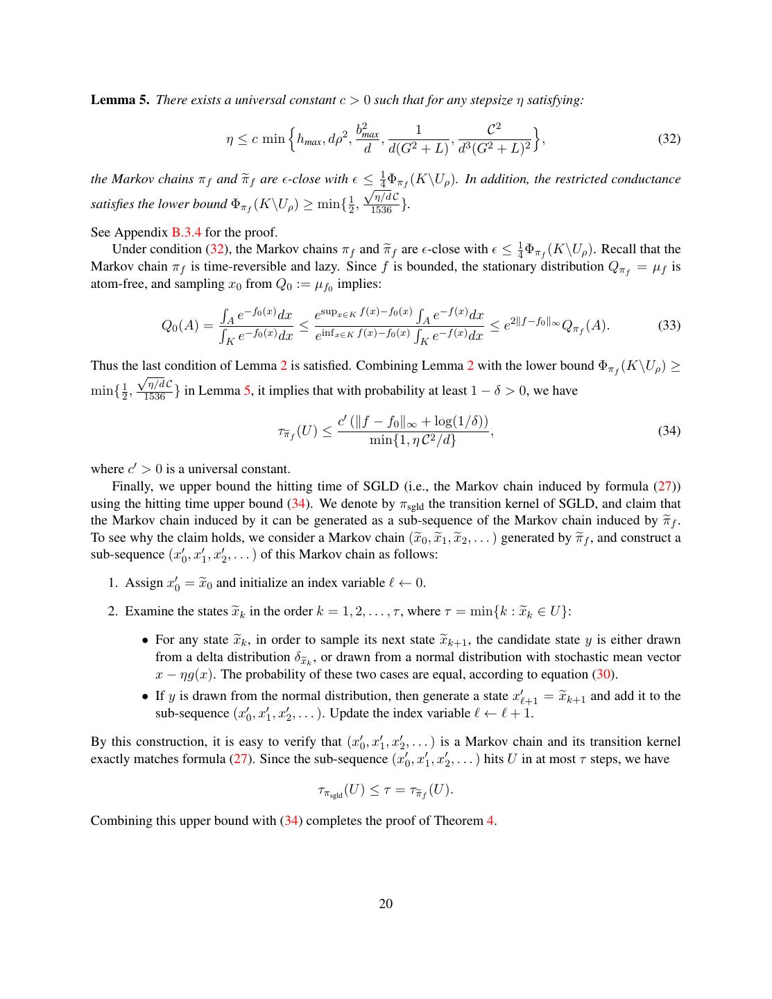
7 .Figure 2: Consider a mapping π : x → x − φ(x). If the conditions of Lemma 1 hold, then we have π(A) ⊂ A and consequentely µf (π(A)) ≤ µf (A ). We use inequality (10) to lower bound the restricted Cheeger constant. The proposition shows that if we choose a big enough ξ, then C(ξf ) (K\U ) will be lower bounded by a universal constant. The lower bound is proved based on an isoperimetric inequality for log-concave distributions. See Appendix C for the proof. For non-convex functions, directly proving the lower bound is difficult, because the definition of C(ξf ) (K\U ) involves verifying the properties of all subsets A ⊂ K\U . We start with a generic lemma that reduces the problem to checking properties of all points in K\U . Lemma 1. Consider an arbitrary continuously differentiable vector field φ : K → Rd and a positive number 0 > 0 such that: φ(x) 2 ≤1 and x − φ(x) ∈ K for any ∈ [0, 0 ], x ∈ K. (9) For any continuously differentiable function f : K → R and any subset V ⊂ K, the restricted Cheeger constant Cf (V ) is lower bounded by d ∂φi (x) Cf (V ) ≥ inf φ(x), ∇f (x) − div φ(x) where div φ(x) := . x∈V ∂xi i=1 Lemma 1 reduces the problem of lower bounding Cf (V ) to the problem of finding a proper vector field φ and verifying its properties for all points x ∈ V . Informally, the quantity Cf (V ) measures the chance of escaping the set V . The lemma shows that if we can construct an “oracle” vector field φ, such that at every point x ∈ V it gives the correct direction (i.e. −φ(x)) to escape V , but always stay in K, then we obtain a strong lower bound on Cf (V ). This construction is merely for the theoretical analysis and doesn’t affect the execution of the algorithm. Proof sketch The proof idea is illustrated in Figure 2: by constructing a mapping π : x → x − φ(x) that satisfies the conditions of the lemma, we obtain π(A) ⊂ A for all A ⊂ V , and consequently µf (π(A)) ≤ µf (A ). Then we are able to lower bound the restricted Cheeger constant by: µf (π(A)) − µf (A) 1 µf (π(dA)) Cf (V ) ≥ lim inf inf = lim inf inf −1 , (10) 0 A⊂V µf (A) 0 dA⊂V µf (dA) where dA is an infinitesimal of the set V . It can be shown that the right-hand side of inequality (10) is equal to inf x∈V { φ(x), ∇f (x) − div φ(x)}, which establishes the lemma. See Appendix D for a rigorous proof. 7 

8 . Before demonstrating the applications of Lemma 1, we make several additional mild assumptions on the parameter space and on the function f . Assumption B (boundary condition and smoothness). • The parameter space K is a d-dimensional ball of radius r > 0 centered at the origin. There exists r0 > 0 such that for every point x satisfying x 2 ∈ [r − r0 , r], we have x, ∇f (x) ≥ x 2 . • For some G, L, H > 0, the function f is third-order differentiable with ∇f (x) 2 ≤ G, ∇2 f (x) ∗ ≤ L and ∇2 f (x) − ∇2 f (y) ∗ ≤ H x − y 2 for any x, y ∈ K. The first assumption requires the parameter space to be an Euclidean ball and imposes a gradient condi- tion on its boundary. This is made mainly for the convenience of theoretical analysis. We remark that for any function f , the condition on the boundary can be satisfied by adding a smooth barrier function ρ( x 2 ) to it, where the function ρ(t) = 0 for any t < r − 2r0 , but sharply increases on the interval [r − r0 , r] to produce large enough gradients. The second assumption requires the function f to be third-order differentiable. We shall relax the second assumption in Section 3. The following proposition describes a lower bound on C(ξf ) (K\U ) when f is a smooth function and the set U consists of approximate stationary points. Although we shall prove a stronger result, the proof of this proposition is a good example for demonstrating the power of Lemma 1. Proposition 2. Assume that Assumption B holds. For any > 0, define the set of -approximate stationary 2 points U := {x ∈ K : ∇f (x) 2 < }. For any ξ ≥ 2L/ 2 , we have C(ξf ) (K\U ) ≥ ξ2G . Proof. Recall that G is the Lipschitz constant of function f . Let the vector field be defined by φ(x) := 1 G ∇f (x), then we have φ(x) 2 ≤ 1. By Assumption B, it is easy to verify that the conditions of Lemma 1 hold. For any x ∈ K\U , the fact that ∇f (x) 2 ≥ implies: ξ ξ 2 φ(x), ξ∇f (x) = ∇f (x) 22 ≥ . G G Recall that L is the smoothness parameter. By Assumption B, the divergence of φ(x) is upper bounded by div φ(x) = G1 tr(∇2 f (x)) ≤ G1 ∇2 f (x) ∗ ≤ G L . Consequently, if we choose ξ ≥ 2L/ 2 as assumed, then we have: ξ 2 L ξ 2 φ(x), ξ∇f (x) − div φ(x) ≥ − ≥ . G G 2G Lemma 1 then establishes the claimed lower bound. Next, we consider approximate local minima [25, 1], which rules out local maxima and strict saddle points. For an arbitrary > 0, the set of -approximate local minima is defined by: √ U := {x ∈ K : ∇f (x) 2 < and ∇2 f (x) − I}. (11) We note that an approximate local minimum is not necessarily close to any local minimum of f . However, if we assume in addition the the function satisfies the (robust) strict-saddle property [14, 20], then any point x ∈ U is guaranteed to be close to a local minimum. Based on definition (11), we prove a lower bound for the set of approximate local minima. Proposition 3. Assume that Assumption B holds. For any > 0, let U be the set of -approximate local minima. For any ξ satisfying max{1, G5/2 L5 , H 5/2 } ξ ≥ O(1) · 2 G1/2 , (12) √ we have C(ξf ) (K\U ) ≥ 8(2G+1)G . The notation O(1) hides a poly-logarithmic function of (L, 1/ ). 8 

9 .Proof sketch Proving Proposition 3 is significantly more challenging than proving Proposition 2. From a high-level point of view, we still construct a vector field φ, then lower bound the expression φ(x), ξ∇f (x) − div φ(x) for every point x ∈ K\U in order to apply Lemma 1. However, there exist saddle points in the set K\U , such that the inner product φ(x), ξ∇f (x) can be very close to zero. For these points, we need to carefully design the vector field so that the term div φ(x) is strictly negative and bounded away from zero. To this end, we define φ(x) to be the sum of two components. The first component aligns with the gradient ∇f (x). The second component aligns with a projected vector Πx (∇f (x)), which projects ∇f (x) to the linear subspace spanned by the eigenvectors of ∇2 f (x) with negative eigenvalues. It can be shown that the second component produces a strictly negative divergence in the neighborhood of strict saddle points. See Appendix E for the complete proof. 2.5 Polynomial-time bound for finding an approximate local minimum Combining Proposition 3 with Theorem 1, we conclude that SGLD finds an approximate local minimum of the function f in polynomial time, assuming that f is smooth enough to satisfy Assumption B. Corollary 1. Assume that Assumptions A,B hold. For an arbitrary > 0, let U be the set of -approximate local minima. For any ρ, δ > 0, there exists a large enough ξ and hyperparameters (η, kmax , D) such that with probability at least 1 − δ, SGLD returns a solution x satisfying f (x) ≤ sup f (x). x: d(x,U )≤ρ The iteration number kmax is bounded by a polynomial function of all hyperparameters in the assumptions as well as ( −1 , ρ−1 , log(1/δ)). Similarly, we can combine Proposition 1 or Proposition 2 with Theorem 1, to obtain complexity bounds for finding the global minimum of a convex function, or finding an approximate stationary point of a smooth function. Corollary 1 doesn’t specify any upper limit on the temperature parameter ξ. As a result, SGLD can be stuck at the worst approximate local minima. It is important to note that the algorithm’s capability of escaping certain local minima relies on a more delicate choice of ξ. Given objective function f , we consider an arbitrary smooth function F such that f − F ∞ ≤ 1/ξ. By Theorem 1, for any target subset U , the hitting time of SGLD can be controlled by lower bounding the restricted Cheeger constant Cξf (K\U ). By the stability property (6), it is equivalent to lower bounding CξF (K\U ) because f and F are uniformly close. If ξ > 0 is chosen large enough (w.r.t. smoothness parameters of F ), then the lower bound established by Proposition 3 guarantees a polynomial hitting time to the set UF of approximate local minima of F . Thus, SGLD can efficiently escape all local minimum of f that lie outside of UF . Since the function F is arbitrary, it can be thought as a favorable perturbation of f such that the set UF eliminates as many local minima of f as possible. The power of such perturbations are determined by their maximum scale, namely the quantity 1/ξ. Therefore, it motivates choosing the smallest possible ξ whenever it satisfies the lower bound in Proposition 3. The above analysis doesn’t specify any concrete form of the function F . In Section 3, we present a concrete analysis where the function F is assumed to be the population risk of empirical risk minimization (ERM). We establish sufficient conditions under which SGLD efficiently finds an approximate local minima of the population risk. 9 

10 .3 Applications to empirical risk minimization In this section, we apply SGLD to a specific family of functions, taking the form: n 1 f (x) := (x; ai ) for x ∈ K. n i=1 These functions are generally referred as the empirical risk in the statistical learning literature. Here, every instance ai ∈ A is i.i.d. sampled from a distribution P, and the function : Rd × A → R measures the loss on individual samples. We define population risk to be the function F (x) := Ex∼P [ (x, a)]. We shall prove that under certain conditions, SGLD finds an approximate local minimum of the (pre- sumably smooth) population risk in polynomial time, even if it is executed on a non-smooth empirical risk. More concretely, we run SGLD on a smoothed approximation of the empirical risk that satisfies Assump- tion A. With large enough sample size, the empirical risk f and its smoothed approximation will be close enough to the population risk F , so that combining the stability property with Theorem 1 and Proposition 3 establishes the hitting time bound. First, let’s formalize the assumptions. Assumption C (parameter space, loss function and population risk). • The parameter space K satisfies: there exists hmax > 0, such that for any x ∈ K and any h ≤ hmax , the random variable y ∼ N (x, 2hI) satisfies P (y ∈ K) ≥ 31 . • There exist ρK , ν > 0 such that in the set K := {x : d(x, K) ≤ ρK }, the population risk F is G-Lipschitz continuous, and supx∈K |f (x) − F (x)| ≤ ν. • For some B > 0, the loss (x; a) is uniformly bounded in [0, B] for any (x, a) ∈ Rd × A. The first assumption is identical to that of Assumption A. The second assumption requires the population risk to be Lipschitz continuous, and it bounds the ∞ -norm distance between f and F . The third assumption requires the loss to be uniformly bounded. Note that Assumption C allows the empirical risk to be non- smooth or even discontinuous. Since the function f can be non-differentiable, the stochastic gradient may not be well defined. We consider a smooth approximation of it following the idea of Duchi et al. [13]: f˜σ (x) := Ez [f (x + z)] where z ∼ N (0, σ 2 Id×d ), (13) where σ > 0 is a smoothing parameter. We can easily compute a stochastic gradient g of f˜σ as follows: z ∇f˜σ (x) = E[g(x) | x] where g(x) := ( (x + z; a) − (x; a)), (14) σ2 Here, z is sampled from N (0, σ 2 Id×d ) and a is uniformly sampled from {a1 , . . . , an }. This stochastic gradient formulation is useful when the loss function is non-differentiable, or when its gradient norms are unbounded. The former happens for minimizing the zero-one loss, and the later can arise in training deep neural networks [26, 6]. Since the loss function is uniformly bounded, formula (14) guarantees that the squared-norm g(x) 22 is sub-exponential. We run SGLD on the function f˜σ . Theorem 1 implies that the time complexity inversely depends on the restricted Cheeger constant C(ξf˜σ ) (K\U ). We can lower bound this quantity using C(ξF ) (K\U ) — the 10 

11 .restricted Cheeger constant of the population risk. Indeed, by choosing a small enough σ, it can be shown that supx∈K |f˜σ (x) − F (x)| ≤ 2ν. The stability property (6) then implies C(ξf˜σ ) (K\U ) ≥ e−4ξν C(ξF ) (K\U ). (15) For any ξ ∈ (0, 1/ν], we have e−4ξν ≥ e−4 , thus the term C(ξf˜σ ) (K\U ) is lower bounded by e−4 C(ξF ) (K\U ). As a consequence, we obtain the following special case of Theorem 1. Theorem 2. Assume that Assumptions C holds. For any subset U ⊂ K, any δ > 0 and any ξ ∈ (0, 1/ν], there exist hyperparameters (η, σ, kmax , D) such that with probability at least 1 − δ, running SGLD on f˜σ returns a solution x satisfying: F (x) ≤ sup F (x) + 5ν. (16) x∈U The iteration number kmax is polynomial in (B, log(1/δ), d, h−1 −1 , ρ−1 , C −1 (K\U )). max , ν K (ξF ) See Appendix F for the proof. In order to lower bound the restricted Cheeger constant C(ξF ) (K\U ), we resort to the general lower bounds in Section 2.4. Consider population risks that satisfy the conditions of Assumption B. By combin- ing Theorem 2 with Proposition 3, we conclude that SGLD finds an approximate local minimum of the population risk in polynomial time. Corollary 2. Assume that Assumption C holds. Also assume that Assumption B holds for the population risk F with smoothness parameters (G, L, H). For any > 0, let U be the set of -approximate local minima of F . If 2 G1/2 sup |f (x) − F (x)| ≤ O(1) · , (17) x∈K max{1, G5/2 L5 , H 5/2 } then there exist hyperparameters (ξ, η, σ, kmax , D) such that with probability at least 1 − δ, running SGLD on f˜σ returns a solution x satisfying F (x) ≤ sup x∈U F (x) + 5ν. The time complexity will be bounded by a polynomial function of all hyperparameters in the assumptions as well as ( −1 , log(1/δ)). The notation O(1) hides a poly-logarithmic function of (L, 1/ ). Assumption B requires the population risk to be sufficiently smooth. Nonetheless, assuming smoothness of the population risk is relatively mild, because even if the loss function is discontinuous, the population risk can be smooth given that the data is drawn from a smooth density. The generalization bound (17) is a necessary condition, because the constraint ξ ≤ 1/ν for Theorem 2 and the constraint (12) for Proposition 3 must simultaneously hold. With a large sample size n, the empirical risk can usually be made sufficiently close to the population risk. There are multiple ways to bound the ∞ -distance between the empirical risk and the population risk, either by bounding the VC-dimension [32], or by bounding the metric entropy [15] or the Rademacher complexity [5] of the function class. We note that for many problems, the function gap uniformly converges to zero in a rate O(n−c ) for some constant c > 0. For such problems, the condition (17) can be satisfied with a polynomial sample complexity. 11 

12 .4 Learning linear classifiers with zero-one loss As a concrete application, we study the problem of learning linear classifiers with zero-one loss. The learner observes i.i.d. training instances (a, b) where (a, b) ∈ Rd × {−1, 1} are feature-label pairs. The goal is to learn a linear classifier a → x, a in order to minimize the zero-one loss:   0 if b × x, a > 0, F (x) := E(a,b)∼P [ (x; (a, b))] where (x; (a, b)) := 1 if b × x, a < 0, 1/2 if x, a = 0,  For a finite dataset {(ai , bi )}ni=1 , the empirical risk is f (x) := n1 ni=1 (x; (ai , bi )). Clearly, the function f is non-convex and discontinous, and has zero gradients almost everywhere. Thus the optimization cannot be accomplished by gradient descent. For a general data distribution, finding a global minimizer of the population risk is NP-hard [3]. We follow Awasthi et al. [4] to assume that the feature vectors are drawn uniformly from the unit sphere, and the observed labels b are corrupted by the Massart noise. More precisely, we assume that there is an unknown unit vector x∗ such that for every feature a ∈ Rd , the observed label b satisfies: 1+q(a) sign( x∗ , a ) with probability 2 ; b= ∗ 1−q(a) (18) −sign( x , a ) with probability 2 ; where 1−q(a) 2 ∈ [0, 0.5] is the Massart noise level. We assume that the noise level is strictly smaller than 0.5 when the feature vector a is separated apart from the decision boundary. Formally, there is a constant 0 < q0 ≤ 1 such that q(a) ≥ q0 | x∗ , a |. (19) The value of q(a) can be adversarially perturbed as long as it satisfies the constraint (19). Awasthi et al. [4] studied the same Massart noise model, but they impose a stronger constraint q(a) ≥ 1 − 3.6 × 10−6 for all a ∈ Rd , so that almost all observed labels are accurate. In contrast, our model (19) captures arbitrary Massart noises (because q0 can be arbitrarily small), and allows for completely random observations at the decision boundary. Our model is thus more general than that of Awasthi et al. [4]. Given function f , we use SGLD to optimize its smoothed approximation (13) in a compact parameter space K := {x ∈ Rd : 1/2 ≤ x 2 ≤ 1}. The following theorem shows that the algorithm finds an approximate global optimum in polynomial time, with a polynomial sample complexity. Theorem 3. Assume that d ≥ 2. For any q0 ∈ (0, 1] and , δ > 0, if the sample size n satisfies: d4 n ≥ O(1) · , q02 4 then there exist hyperparameters (ξ, η, σ, kmax , D) such that SGLD on the smoothed function (13) returns a solution x satisfying F (x) ≤ F (x∗ ) + with probability at least 1 − δ. The notation O(1) hides a poly-logarithmic function of (d, 1/q0 , 1/ , 1/δ). The time complexity of the algorithm is polynomial in (d, 1/q0 , 1/ , log(1/δ)). 12 

13 .Proof sketch The proof consists of two parts. For the first part, we prove that the population risk is Lipschitz continuous and the empirical risk uniformly converges to the population risk, so that Assumption C hold. For the second part, we lower bound the restricted Cheeger constant by Lemma 1. The proof is spiritually similar to that of Proposition 2 or Proposition 3. We define U to be the set of approximately optimal solutions, and construct a vector field φ such that: φ(x) ∝ x, x∗ x − x 2 ∗ 2x . By lower bounding the expression φ(x), ∇f (x) −div φ(x) for all x ∈ K\U , Lemma 1 establishes a lower bound on the restricted Cheeger constant. The theorem is established by combining the two parts together and by Theorem 2. We defer the full proof to Appendix G. 5 Conclusion In this paper, we analyzed the hitting time of the SGLD algorithm on non-convex functions. Our approach is different from existing analyses on Langevin dynamics [10, 12, 8, 30, 27], which connect LMC to a continuous-time Langevin diffusion process, then study the mixing time of the latter process. In contrast, we are able to establish polynomial-time guarantees for achieving certain optimality sets, regardless of the exponential mixing time. For future work, we hope to establish stronger results on non-convex optimization using the techniques developed in this paper. Our current analysis doesn’t apply to training over-specified models. For these models, the empirical risk can be minimized far below the population risk [29], thus the assumption of Corollary 2 is violated. In practice, over-specification often makes the optimization easier, thus it could be interesting to show that this heuristic actually improves the restricted Cheeger constant. Another open problem is avoiding poor population local minima. Jin et al. [16] proved that there are many poor population local minima in training Gaussian mixture models. It would be interesting to investigate whether a careful initialization could prevent SGLD from hitting such bad solutions. References [1] N. Agarwal, Z. Allen-Zhu, B. Bullins, E. Hazan, and T. Ma. Finding local minima for nonconvex optimization in linear time. arXiv preprint arXiv:1611.01146, 2016. [2] A. Anandkumar and R. Ge. Efficient approaches for escaping higher order saddle points in non-convex optimization. arXiv preprint arXiv:1602.05908, 2016. [3] S. Arora, L. Babai, J. Stern, and Z. Sweedyk. The hardness of approximate optima in lattices, codes, and systems of linear equations. In Foundations of Computer Science, 1993. Proceedings., 34th Annual Symposium on, pages 724–733. IEEE, 1993. [4] P. Awasthi, M. Balcan, N. Haghtalab, and R. Urner. Efficient learning of linear separators under bounded noise. In Proceedings of the 28th Conference on Learning Theory, 2015. [5] P. L. Bartlett and S. Mendelson. Rademacher and Gaussian complexities: Risk bounds and structural results. The Journal of Machine Learning Research, 3:463–482, 2003. 13 

14 . [6] Y. Bengio, N. Boulanger-Lewandowski, and R. Pascanu. Advances in optimizing recurrent networks. In 2013 IEEE International Conference on Acoustics, Speech and Signal Processing, pages 8624– 8628. IEEE, 2013. [7] A. L. Blum and R. L. Rivest. Training a 3-node neural network is NP-complete. Neural Networks, 5 (1):117–127, 1992. [8] T. Bonis. Guarantees in wasserstein distance for the langevin monte carlo algorithm. arXiv preprint arXiv:1602.02616, 2016. [9] A. Bovier, M. Eckhoff, V. Gayrard, and M. Klein. Metastability in reversible diffusion processes i: Sharp asymptotics for capacities and exit times. Journal of the European Mathematical Society, 6(4): 399–424, 2004. [10] S. Bubeck, R. Eldan, and J. Lehec. Finite-time analysis of projected langevin monte carlo. In Advances in Neural Information Processing Systems, pages 1243–1251, 2015. [11] J. Cheeger. A lower bound for the smallest eigenvalue of the laplacian. 1969. [12] A. S. Dalalyan. Theoretical guarantees for approximate sampling from smooth and log-concave den- sities. Journal of the Royal Statistical Society: Series B (Statistical Methodology), 2016. [13] J. C. Duchi, M. I. Jordan, M. J. Wainwright, and A. Wibisono. Optimal rates for zero-order convex optimization: the power of two function evaluations. IEEE Transactions on Information Theory, 61 (5):2788–2806, 2015. [14] R. Ge, F. Huang, C. Jin, and Y. Yuan. Escaping from saddle pointsonline stochastic gradient for tensor decomposition. In Proceedings of The 28th Conference on Learning Theory, pages 797–842, 2015. [15] D. Haussler. Decision theoretic generalizations of the pac model for neural net and other learning applications. Information and computation, 100(1):78–150, 1992. [16] C. Jin, Y. Zhang, S. Balakrishnan, M. J. Wainwright, and M. I. Jordan. On local maxima in the population likelihood of gaussian mixture models: Structural results and algorithmic consequences. In Advances In Neural Information Processing Systems, pages 4116–4124, 2016. [17] Ł. Kaiser and I. Sutskever. Neural gpus learn algorithms. arXiv preprint arXiv:1511.08228, 2015. [18] K. Kurach, M. Andrychowicz, and I. Sutskever. Neural random-access machines. arXiv preprint arXiv:1511.06392, 2015. [19] B. Laurent and P. Massart. Adaptive estimation of a quadratic functional by model selection. Annals of Statistics, pages 1302–1338, 2000. [20] J. D. Lee, M. Simchowitz, M. I. Jordan, and B. Recht. Gradient descent converges to minimizers. University of California, Berkeley, 1050:16, 2016. [21] P.-L. Loh and M. J. Wainwright. Regularized m-estimators with nonconvexity: statistical and algorith- mic theory for local optima. The Journal of Machine Learning Research, 16(1):559–616, 2015. [22] L. Lov´asz and M. Simonovits. Random walks in a convex body and an improved volume algorithm. Random structures & algorithms, 4(4):359–412, 1993. 14 

15 .[23] A. Neelakantan, Q. V. Le, and I. Sutskever. Neural programmer: Inducing latent programs with gradi- ent descent. arXiv preprint arXiv:1511.04834, 2015. [24] A. Neelakantan, L. Vilnis, Q. V. Le, I. Sutskever, L. Kaiser, K. Kurach, and J. Martens. Adding gradient noise improves learning for very deep networks. arXiv preprint arXiv:1511.06807, 2015. [25] Y. Nesterov and B. T. Polyak. Cubic regularization of newton method and its global performance. Mathematical Programming, 108(1):177–205, 2006. [26] R. Pascanu, T. Mikolov, and Y. Bengio. On the difficulty of training recurrent neural networks. ICML (3), 28:1310–1318, 2013. [27] M. Raginsky, A. Rakhlin, and M. Telgarsky. Non-convex learning via stochastic gradient langevin dynamics: a nonasymptotic analysis. 2017. [28] G. O. Roberts and R. L. Tweedie. Exponential convergence of langevin distributions and their discrete approximations. Bernoulli, pages 341–363, 1996. [29] I. Safran and O. Shamir. On the quality of the initial basin in overspecified neural networks. arXiv preprint arXiv:1511.04210, 2015. [30] Y. W. Teh, A. H. Thiery, and S. J. Vollmer. Consistency and fluctuations for stochastic gradient langevin dynamics. Journal of Machine Learning Research, 17(7):1–33, 2016. [31] Y. L. Tong. The multivariate normal distribution. Springer Science & Business Media, 2012. [32] V. N. Vapnik. An overview of statistical learning theory. IEEE transactions on neural networks, 10 (5):988–999, 1999. [33] Z. Wang, H. Liu, and T. Zhang. Optimal computational and statistical rates of convergence for sparse nonconvex learning problems. Annals of statistics, 42(6):2164, 2014. [34] M. Welling and Y. W. Teh. Bayesian learning via stochastic gradient langevin dynamics. In Proceed- ings of the 28th International Conference on Machine Learning, pages 681–688, 2011. [35] A. Zeyer, P. Doetsch, P. Voigtlaender, R. Schl¨uter, and H. Ney. A comprehensive study of deep bidi- rectional lstm rnns for acoustic modeling in speech recognition. arXiv preprint arXiv:1606.06871, 2016. A Restricted Cheeger constant is strictly positive In this appendix, we prove that under mild conditions, the restricted Cheeger constant for a convex parameter space is always strictly positive. Let K be an arbitrary convex parameter space with diameter D < +∞. Lov´asz and Simonovits [22, Theorem 2.6] proved the following isoperimetric inequality: for any subset A ⊂ K and any > 0, the following lower bound holds: vol(A ) − vol(A) 2 ≥ , (20) min{vol(A), vol(K\A )} D 15 

16 .where vol(A) represents the Borel measure of set A. Let f0 (x) := 0 be a constant zero function. By the definition of the function-induced probability measure, we have vol(A) µf0 (A) = for all A ⊂ K. (21) vol(K) Combining the inequality (20) with equation (21), we obtain: µf0 (A ) − µf0 (A) µf0 (A ) − µf0 (A) 2 ≥ ≥ . µf0 (A) (1 − µf0 (A )) min{µf0 (A), 1 − µf0 (A )} D If the set A satisfies A ⊂ V ⊂ K, then 1 − µf0 (A ) ≥ 1 − µf0 (V ). Combining it with the above inequality, we obtain: µf0 (A ) − µf0 (A) 2(1 − µf0 (V )) 2(vol(K) − vol(V )) ≥ = . µf0 (A) D D vol(K) According to the definition of the restricted Cheeger constant, the above lower bound implies: 2(vol(K) − lim →0 vol(V )) Cf0 (V ) ≥ . (22) D vol(K) Consider an arbitrary bounded function f satisfying supx∈K |f (x)| ≤ B < +∞, combining the stability property (6) and inequality (22), we obtain: 2(vol(K) − lim →0 vol(V )) Cf (V ) ≥ e−2B × . D vol(K) We summarize the result as the following proposition. Proposition 4. Assume that K is a convex parameter space with finite diameter. Also assume that V ⊂ K is a measurable set satisfying lim →0 vol(V ) < vol(K). For any bounded function f : K → R, the restricted Cheeger constant Cf (V ) is strictly positive. B Proof of Theorem 1 The proof consists of two parts. We first establish a general bound on the hitting time of Markov chains to a certain subset U ⊂ K, based on the notion of restricted conductance. Then we prove that the hitting time of SGLD can be bounded by the hitting time of a carefully constructed time-reversible Markov chain. This Markov chain runs a Metropolis-Hastings algorithm that converges to the stationary distribution µξf . We prove that this Markov chain has a bounded restricted conductance, whose value is characterized by the restricted Cheeger constant that we introduced in Section 2.2. Combining the two parts establishes the general theorem. B.1 Hitting time of Markov chains For an arbitrary Markov chain defined on the parameter space K, we represent the Markov chain by its transition kernel π(x, A), which gives the conditional probability that the next state satisfies xk+1 ∈ A given the current state xk = x. Similarly, we use π(x, x ) to represent the conditional probability P (xk+1 = x |xk = x). If π has a stationary distribution, then we denote it by Qπ . 16 

17 . A Markov chain is call lazy if π(x, x) ≥ 1/2 for every x ∈ K, and is called time-reversible if it satisfies π(x, B)Qπ (x) = π(x, A)Qπ (x) for any A, B ⊂ K. A B If (x0 , x1 , x2 , . . . ) is a realization of the Markov chain π, then the hitting time to some set U ⊂ K is denoted by: τπ (U ) := min{k : xk ∈ U }. For arbitrary subset V ⊂ K, we define the restricted conductance, denoted by Φπ (V ), to be the follow- ing infinimum ratio: A π(x, K\A)Qπ (x)dx Φπ (V ) := inf . (23) A⊂V Qπ (A) Based on the notion of restricted conductance, we present a general upper bound on the hitting time. For arbitrary subset U ⊂ K, suppose that π is an arbitrary Markov chain whose transition kernel is stationary inside U , namely it satisfies π(x, x) = 1 for any x ∈ U . Let (x0 , x1 , x2 , . . . ) be a realization of the Markov chain π. We denote by Qk the probability distribution of xk at iteration k. In addition, we define a measure of closeness between any two Markov chains. Definition. For two Markov chains π and π, we say that π is -close to π w.r.t. a set U if the following condition holds for any x ∈ K\U and any A ⊂ K\{x}: π(x, A) ≤ π(x, A) ≤ (1 + )π(x, A). (24) Then we are able to prove the following lemma. Lemma 2. Let π be a time-reversible lazy Markov chain with atom-free stationary distribution Qπ . Assume that π is -close to π w.r.t. U where ≤ 41 Φπ (K\U ). If there is a constant M such that the distribution Q0 satisfies Q0 (A) ≤ M Qπ (A) for any A ⊂ K\U , then for any δ > 0, the hitting time of the Markov chain is bounded by: 4 log(M/δ) τπ (U ) ≤ , (25) Φ2π (K\U ) with probability at least 1 − δ. See Appendix B.3.1 for the proof of Lemma 2. The lemma shows that if the two chains π and π are sufficiently close, then the hitting time of the Markov chain π will be inversely proportional to the square of the restricted conductance of the Markov chain π, namely Φπ (K\U ). Note that if the density function of distribution Qπ is bounded, then by choosing Q0 to be the uniform distribution over K, there exists a finite constant M such that Q0 (A) ≤ M Qπ (A), satisfying the last condition of Lemma 2. B.2 Proof of the theorem The SGLD algorithm initializes x0 by the uniform distribution µf0 (with f0 (x) ≡ 0). Then at iteration k ≥ 1, it performs the following update: yk if yk ∈ K ∩ B(xk−1 ; 4 2ηd/ξ), yk = xk−1 − η · g(xk−1 ) + 2η/ξ · w; xk = (26) xk−1 otherwise. 17 

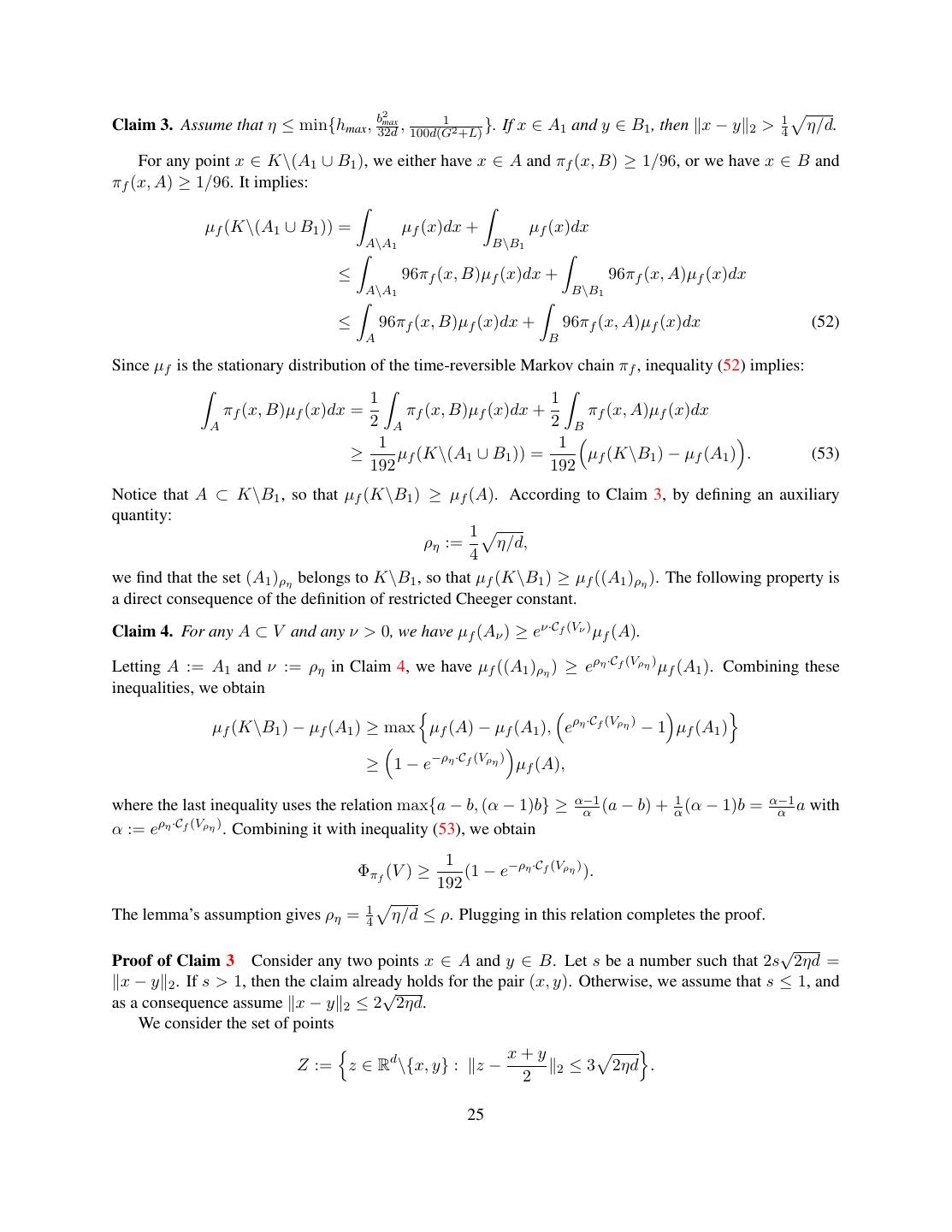
18 .We refer the particular setting ξ = 1 as the “standard setting”. For the “non-standard” setting of ξ = 1, we rewrite the first equation as: yk = xk−1 − (η/ξ) · (ξg(xk−1 )) + 2(η/ξ) · w. This re-formulation reduces to the problem to the standard setting, with stepsize η/ξ and objective func- tion ξf . Thus it suffices to prove the theorem in the standard setting, then plug in the stepsize η/ξ and the objective function ξf to obtain the general theorem. Therefore, we assume ξ = 1 and consider the sequence of points (x0 , x1 , . . . ) generated by: √ yk if yk ∈ K ∩ B(xk−1 ; 4 2ηd), yk = xk−1 − η · g(xk−1 ) + 2η · w; xk = (27) xk−1 otherwise. We introduce two additional notations: for arbitrary functions f1 , f2 , we denote the maximal gap supx∈K |f1 (x) − f2 (x)| by the shorthand f1 − f2 ∞ . For arbitrary set V ⊂ K and ρ > 0, we denote the super-set {x ∈ K : d(x, V ) ≤ ρ} by the shorthand Vρ . Then we prove the following theorem for the standard setting. Theorem 4. Assume that Assumption A holds. Let x0 be sampled from µf0 and let the Markov chain (x0 , x1 , x2 , · · · ) be generated by update (27). Let U ⊂ K be an arbitrary subset and let ρ > 0 be an arbitrary positive number. Let C := Cf (K\U ) be a shorthand notation. Then for any δ > 0 and any stepsize η satisfying b2max 1 C2 η ≤ c min dρ2 , hmax , , , , (28) d d(G2 + L) d3 (G2 + L)2 the hitting time to set Uρ is bounded by c f − f0 ∞ + log(1/δ) min{k : xk ∈ Uρ } ≤ , (29) min{1, η C 2 /d} with probability at least 1 − δ. Here, c, c > 0 are universal constants. Theorem 4 shows that if we choose η ∈ (0, η0 ], where η0 is the right-hand side of inequality (28), then with probability at least 1 − δ, the hitting time to the set Uρ is bounded by c d B + log(1/δ) c B + log(1/δ) min{k : xk ∈ Uρ } ≤ 2 = . ηC min{1, (η/η0 ) η0 C 2 /d} Combining it with the definition of η0 , and with simple algebra, we conclude that min{k : xk ∈ Uρ } ≤ M min{1,C}4 where M is polynomial in (B, L, G, log(1/δ), d, η0 /η, h−1 −1 −1 max , bmax , ρ ). This establishes the iter- ation complexity bound. Whenever xk hits Uρ , we have f (x) ≤ f (xk ) ≤ sup f (x), x: d(x,U )≤ρ which establishes the risk bound. Thus, Theorem 4 establishes Theorem 1 for the special case of ξ = 1. In the non-standard setting (ξ = 1), we follow the reduction described above to substitute (η, f ) in Theorem 4 with the pair (η/ξ, ξf ). As a consequence, the quantity C is substituted with C(ξf ) (K\U ), and (B, L, G, η0 , bmax ) are substituted with (ξB, ξL, ξG, η0 /ξ, bmax /ξ). Both the iteration complexity bound and the risk bound hold as in the standard setting, except that after the substitution, the numerator M in the iteration complexity bound has an additional polynomial dependence on ξ. Thus we have proved the general conclusion of Theorem 1. 18 

19 .Proof of Theorem 4 For the function f : K → Rd satisfying Assumption A, we define a time-reversible Markov chain represented by the following transition kernel πf . Given any current state xk = x ∈ K, the Markov chain draws a “candidate state” y ∈ Rd from the following the density function: y−x+η·g(x) 2 1 1 1 − 2 qx (y) := δx (y) + · d/2 E e 4η |x (30) 2 2 (4πη) where δx is the Dirac delta function at point x. The expectation is taken over the stochastic gradient g √ defined in equation (27), conditioning on the current state x. Then for any candidate state y ∈ K ∩ B(x; 4 2ηd), we accept the candidate state (i.e., xk+1 = y) with probability: qy (x) f (x)−f (y) αx (y) := min 1, e , (31) qx (y) √ the candidate state (i.e., xk+1 = x) with probability 1 − αx (y). All candidate states y ∈ or reject / K∩ B(x; 4 2ηd) are rejected (i.e., xk+1 = x). It is easy to verify that πf executes a Metropolis-Hastings algorithm. Therefore, it induces a time-reversible Markov chain, and its stationary distribution is equal to µf (x) ∝ e−f (x) . Given the subset Uρ ⊂ K, we define an auxiliary Markov chain and its transition kernel πf as follow. Given any current state xk = x ∈ K, the Markov chain proposes a candidate state y ∈ Rd through the density function qx (y)√ defined by equation (30), then accepts the candidate state if and only if x ∈ / Uρ and y ∈ K ∩ B(x; 4 2ηd). Upon acceptance, the next state of πf is defined to be xk+1 = y, otherwise xx+1 = x. The Markov chains πf differs from πf only in their different probabilities for acccepting the √∈ Uρ , then πf may accept y with probability αx (y), but πf always rejects y. If x ∈ candidate state y. If x / Uρ and y ∈ K ∩ B(x; 4 2ηd), then πf accepts y with probability αx (y), while πf accepts with probability 1. Despite the difference in their definitions, we are able to show that the two Markov chains are -close, where depends on the stepsize η and the properties of the objective function. 2 Lemma 3. Assume that 0 < η ≤ b32d max and Assumption A hold. Then the Markov chain πf is -close to πf 33ηd(G 2 +L) w.r.t. Uρ with = e − 1. See Appendix B.3.2 for the proof. Lemma 3 shows that if we choose η small enough, then will be sufficiently small. Recall from Lemma 2 that we need ≤ 14 Φπf (K\Uρ ) to bound the Markov chain πf ’s hitting time to the set Uρ . It means that η has to be chosen based on the restricted conductance of the Markov chain πf . Although calculating the restricted conductance of a Markov chain might be difficult, the following lemma shows that the restricted conductance can be lower bounded by the restricted Cheeger constant. 2 Lemma 4. Assume that η ≤ min{hmax , 16dρ2 , b32d max , 100d(G1 2 +L) } and Assumption A hold. Then for any V ⊂ K, we have: √ 1 1 Φπf (V ) ≥ (1 − e− 4 η/d Cf (Vρ ) ). 192 See Appendix B.3.3 for the proof. By Lemma 3 and Lemma 4, we are able to choose a sufficiently small η such that the Markov chains πf and πf are close enough to satisfy the conditions of Lemma 2. Formally, the following condition on η is sufficient. 19 

20 .Lemma 5. There exists a universal constant c > 0 such that for any stepsize η satisfying: b2max 1 C2 η ≤ c min hmax , dρ2 , , , , (32) d d(G2 + L) d3 (G2 + L)2 the Markov chains πf and πf are -close with ≤ 14 Φπf (K\Uρ ). In addition, the restricted conductance √ 1 η/d C satisfies the lower bound Φπf (K\Uρ ) ≥ min{ 2 , 1536 }. See Appendix B.3.4 for the proof. Under condition (32), the Markov chains πf and πf are -close with ≤ 41 Φπf (K\Uρ ). Recall that the Markov chain πf is time-reversible and lazy. Since f is bounded, the stationary distribution Qπf = µf is atom-free, and sampling x0 from Q0 := µf0 implies: −f0 (x) dx esupx∈K f (x)−f0 (x) −f (x) dx Ae Ae f −f0 Q0 (A) = −f0 (x) dx ≤ −f (x) dx ≤ e2 ∞ Qπf (A). (33) Ke einf x∈K f (x)−f0 (x) Ke Thus the last condition of Lemma 2 is satisfied. Combining Lemma 2 with the lower bound Φπf (K\Uρ ) ≥ √ 1 η/d C min{ 2 , 1536 } in Lemma 5, it implies that with probability at least 1 − δ > 0, we have c ( f − f0 ∞ + log(1/δ)) τπf (U ) ≤ , (34) min{1, η C 2 /d} where c > 0 is a universal constant. Finally, we upper bound the hitting time of SGLD (i.e., the Markov chain induced by formula (27)) using the hitting time upper bound (34). We denote by πsgld the transition kernel of SGLD, and claim that the Markov chain induced by it can be generated as a sub-sequence of the Markov chain induced by πf . To see why the claim holds, we consider a Markov chain (x0 , x1 , x2 , . . . ) generated by πf , and construct a sub-sequence (x0 , x1 , x2 , . . . ) of this Markov chain as follows: 1. Assign x0 = x0 and initialize an index variable ← 0. 2. Examine the states xk in the order k = 1, 2, . . . , τ , where τ = min{k : xk ∈ U }: • For any state xk , in order to sample its next state xk+1 , the candidate state y is either drawn from a delta distribution δxk , or drawn from a normal distribution with stochastic mean vector x − ηg(x). The probability of these two cases are equal, according to equation (30). • If y is drawn from the normal distribution, then generate a state x +1 = xk+1 and add it to the sub-sequence (x0 , x1 , x2 , . . . ). Update the index variable ← + 1. By this construction, it is easy to verify that (x0 , x1 , x2 , . . . ) is a Markov chain and its transition kernel exactly matches formula (27). Since the sub-sequence (x0 , x1 , x2 , . . . ) hits U in at most τ steps, we have τπsgld (U ) ≤ τ = τπf (U ). Combining this upper bound with (34) completes the proof of Theorem 4. 20 

21 .B.3 Proof of technical lemmas B.3.1 Proof of Lemma 2 Let q := Qπ (K\U ) be a shorthand notation. Let Gp be the class of functions g : K\U → [0, 1] such that K\U g(x)Qπ (x)dx = p. We define a sequence of functions hk : [0, q] → R (k = 1, 2, . . . ) such that hk (p) := sup g(x)Qk (x)dx. (35) g∈Gp K\U By its definition, the function hk is a concave function on [0, q]. In addition, [22, Lemma 1.2] proved the following properties for the function hk : if Qπ is atom-free, then for any p ∈ [0, q] there exists a function g(x) := I(x ∈ A) that attains the supremum in the definition of hk . We claim the following property of the function hk . √ Claim 1. If there is a constant C such that the inequality h0 (p) ≤ C p holds for any p ∈ [0, q], then the inequality √ 1 hk (p) ≤ C p(1 − Φ2π (K\U ))k (36) 4 holds for any k ∈ N and any p ∈ [0, q]. According to the claim, it suffices to upper bound h0 (p) for p ∈ [0, q]. Indeed, since Q0 (A) ≤ M Qπ (A) for any A ⊂ K\U , we immediately have: √ h0 (p) = sup Q0 (A) ≤ M p ≤ M p. A⊂K\U : Qπ (A)=p Thus, we have 1 Qk (K\U ) ≤ hk (q) ≤ M (1 − Φ2π (K\U ))k . 4 Choosing k := 4Φlog(M/δ) 2 (K\U ) implies Qk (K\U ) ≤ δ. As a consequence, the hitting time is bounded by k with π probability at least 1 − δ. Proof of Claim 1 Recall the properties of the function hk . For any p ∈ [0, q], we can find a set A ⊂ K\U such that Qπ (A) = p and hk (p) = Qk (A). Define, for x ∈ K, two functions: 2π(x, A) − 1 if x ∈ A g1 (x) = , 0 if x ∈ /A 1 if x ∈ A g2 (x) = ., 2π(x, A) if x ∈ /A By the laziness of the Markov chain π, we obtain 0 ≤ gi ≤ 1, so that they are functions mapping from K\U to [0, 1]. Using the relation 2π(x, A) − 1 = 1 − 2π(x, K\A), the definition of g1 implies that: g1 (x)Qπ (x)dx = Qπ (A) − 2 π(x, K\A)Qπ (x)dx = p − 2 π(x, K\A)Qπ (x)dx K\U A A ≤p−2 π(x, K\A)Qπ (x)dx. (37) A 21 

22 .where the last inequality follows since the δ-closeness ensures π(x, K\A) ≤ π(x, K\A). Similarly, using the definition of g2 and the relation π(x, A) ≤ (1 + )π(x, A), we obtain: g2 (x)Qπ (x)dx = Qπ (A) + 2 π(x, A)Qπ (x)dx K\U K\(U ∪A) ≤p+2 π(x, A)Qπ (x)dx K\A ≤p+2 (1 + )π(x, A)Qπ (x)dx (38) K\A Since Qπ is the stationary distribution of the time-reversible Markov chain π, the right-hand side of (38) is equal to: p+2 (1 + )π(x, A)Qπ (x)dx = p + 2(1 + ) π(x, K\A)Qπ (x)dx (39) K\A A Let p1 and p2 be the left-hand side of inequality (37) and (38) respectively, and define a shorthand notation: 1 r := π(x, K\A)Qπ (x)dx. p A Then by definition of restricted conductance and the laziness of π, we have Φπ (K\U ) ≤ r ≤ 1/2. Com- bining inequalities (37), (38) and (39) and by simple algebra, we obtain: √ √ √ √ √ p1 + p2 ≤ p 1 − 2r + 1 + 2 r + 2r . By the condition ≤ 41 Φπ (K\U ) ≤ 4r , the above inequality implies √ √ √ √ p1 + p2 ≤ p 1 − 2r + 1 + 2r + r2 /2 √ It is straightforward to verify that for any 0 ≤ r ≤ 1, the right-hand side is upper bounded by 2(1−r2 /4) p. Thus we obtain: √ √ √ p1 + p2 ≤ 2(1 − r2 /4) p. (40) On the other hand, the definition of g1 and g2 implies that π(x, A) = g1 (x)+g 2 2 (x) for any x ∈ K\U . For all x ∈ U , the transition kernel π is stationary, so that we have π(x, A) = 0. Combining these two facts implies hk (p) = Qk (A) = π(x, A)Qk−1 (x)dx K\U 1 1 = g1 (x)Qk−1 (x)dx + g2 (x)Qk−1 (x)dx ≤ (hk−1 (p1 ) + hk−1 (p2 )). (41) 2 K\U K\U 2 The last inequality uses the definition of function hk−1 . 22 

23 . Finally, we prove inequality (36) by induction. The inequality holds for k = 0 by the assumption. We assume by induction that it holds for an aribtrary integer k − 1, and prove that it holds for k. Combining the inductive hypothesis with inequalities (40) and (41), we have C √ √ 1 √ 1 hk (p) ≤ ( p1 + p2 )(1 − Φ2π (K\U ))k−1 ≤ C p(1 − r2 /4)(1 − Φ2π (K\U ))k−1 2 4 4 √ 1 2 ≤ C p(1 − Φπ (K\U ))k , 4 Thus, inequality (36) holds for k, which completes the proof. B.3.2 Proof of Lemma 3 By the definition of the -closeness, it suffices to consider an arbitrary x ∈ / Uρ and verify the inequality (24). √ ratio of πf and πf are different, that is, when the candidate state y We focus on cases when the acceptance satisfies y = x and y ∈ K ∩ B(x; 4 2ηd). We make the following claim on the acceptance ratio. 2 √ Claim 2. For any 0 < η ≤ b32d max , if we assume x ∈ / Uρ , y ∈ / x, and y ∈ K ∩ B(x; 4 2ηd), then the 2 acceptance ratio is lower bounded by αx (y) ≥ e−33ηd(G +L) . Consider an arbitrary point x ∈ K\Uρ and an arbitrary subset A ⊂ K\{x}. The definitions of πf and πf imply that πf (x, A) ≤ πf (x, A) always hold. In order to prove the opposite, we notice that: πf (x, A) = √ qx (y)dy. (42) A∩B(x;4 2ηd) The definition of πf and Claim 2 implies 2 +L) √ qx (y)dy ≤ e33ηd(G √ qx (y)αx (y)dy A∩B(x;4 2ηd) A∩B(x;4 2ηd) 2 +L) = e33ηd(G π(x, A), which completes the proof. Proof of Claim 2 By plugging in the definition of αx (y) and αy (x) and the fact that x = y, we obtain x−y+η·g(y) 2 2 − qy (x) f (x)−f (y) E[e 4η | y] e = y−x+η·g(x) 2 · ef (x)−f (y) . (43) qx (y) − 2 E[e 4η | x] In order to prove the claim, we need to lower bound the numerator and upper bound the denominator of equation (43). For the numerator, Jensen’s inequality implies: x−y+η·g(y) 2 2 x−y+η·g(y) 2 2 |y] x−y 2 2 −E[ x−y, g(y) η g(y) 2 2 |y] − −E[ − + E e 4η |y ≥e 4η =e 4η 2 4 x−y 2 2 − x−y, ∇f (y) 2 − − ηdG ≥e 4η 2 4 (44) 23 

24 .where the last inequality uses the upper bound d d 1 1 2 E[ g(y) 22 |y] = E[(bmax gi (y))2 |y] ≤ log E[e(bmax gi (y)) |y] b2max b2max i=1 i=1 d 1 2 b2 ≤ log eG max = dG2 . (45) b2max i=1 For the above deduction, we have used the Jensen’s inequality as well as Assumption A. For the denominator, we notice that the term inside the expectation satisfies: y−x+η·g(x) 2 2 x−y 2 2 − y−x, g(x) e− 4h ≤ e− 4h 2 (46) y−x, g(x) 2 Let X be a shorthand for the random variable 2 . Using the relation that et ≤ t + et holds for all t ∈ R, we have 2 E[eX ] = eE[X] E[eX−E[X] ] = eE[X] E[eX−E[X] − (X − E[X])] ≤ eE[X] E[e(X−E[X]) ]. (47) For the second term on the righthand side, using the relation (a − b)2 ≤ 2a2 + 2b2 and Jensen’s inequality, we obtain 2 2 2 2 2 2 2 E[e(X−E[X]) ] ≤ E[e2X +2(E[X]) ] = E[e2X ] · e2(E[X]) ≤ (E[e2X ])2 ≤ E[e4X ], (48) √ Since x − y 2 ≤ 4 2ηd ≤ bmax is assumed, Assumption A implies 2 x−y, g(x) )2 2 2 2 E[e4X ] = E[e( ] ≤ eG x−y 2 ≤ e32ηdG . (49) Combining inequalities (46)-(49), we obtain y−x+η·g(x) 2 x−y 2 2 − y−x, ∇f (x) 2 +32ηdG2 E e− 4h | x ≤ e− 4h 2 . (50) Combining equation (43) with inequalities (44), (50), we obtain qy (x) f (x)−f (y) ∇f (x)+∇f (y) −33ηdG2 e ≥ ef (x)−f (y)− x−y, 2 . (51) qx (y) The L-smoothness of function f implies that ∇f (x) + ∇f (y) L x−y 2 2 f (x) − f (y) − x − y, ≥− ≥ −16ηdL. 2 2 Combining this inequality with the lower bound (51) completes the proof. B.3.3 Proof of Lemma 4 Recall that µf is the stationary distribution of the Markov chain πf . We consider an arbitrary subset A ⊂ V , and define B := K\A. Let A1 and B1 be defined as A1 := {x ∈ A : πf (x, B) < 1/96} and B1 := {x ∈ B : πf (x, A) < 1/96}, In other words, the points in A1 and B1 have low probability to move across the broader between A and B. We claim that the distance between points in A1 and B1 must be bounded away from a positive number. 24 

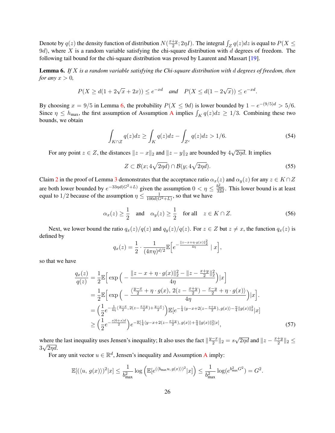
25 . 2 Claim 3. Assume that η ≤ min{hmax , b32d max 1 , 100d(G 2 +L) }. If x ∈ A1 and y ∈ B1 , then x − y 2 > 1 4 η/d. For any point x ∈ K\(A1 ∪ B1 ), we either have x ∈ A and πf (x, B) ≥ 1/96, or we have x ∈ B and πf (x, A) ≥ 1/96. It implies: µf (K\(A1 ∪ B1 )) = µf (x)dx + µf (x)dx A\A1 B\B1 ≤ 96πf (x, B)µf (x)dx + 96πf (x, A)µf (x)dx A\A1 B\B1 ≤ 96πf (x, B)µf (x)dx + 96πf (x, A)µf (x)dx (52) A B Since µf is the stationary distribution of the time-reversible Markov chain πf , inequality (52) implies: 1 1 πf (x, B)µf (x)dx = πf (x, B)µf (x)dx + πf (x, A)µf (x)dx A 2A 2 B 1 1 ≥ µf (K\(A1 ∪ B1 )) = µf (K\B1 ) − µf (A1 ) . (53) 192 192 Notice that A ⊂ K\B1 , so that µf (K\B1 ) ≥ µf (A). According to Claim 3, by defining an auxiliary quantity: 1 ρη := η/d, 4 we find that the set (A1 )ρη belongs to K\B1 , so that µf (K\B1 ) ≥ µf ((A1 )ρη ). The following property is a direct consequence of the definition of restricted Cheeger constant. Claim 4. For any A ⊂ V and any ν > 0, we have µf (Aν ) ≥ eν·Cf (Vν ) µf (A). Letting A := A1 and ν := ρη in Claim 4, we have µf ((A1 )ρη ) ≥ eρη ·Cf (Vρη ) µf (A1 ). Combining these inequalities, we obtain µf (K\B1 ) − µf (A1 ) ≥ max µf (A) − µf (A1 ), eρη ·Cf (Vρη ) − 1 µf (A1 ) ≥ 1 − e−ρη ·Cf (Vρη ) µf (A), α−1 1 α−1 where the last inequality uses the relation max{a − b, (α − 1)b} ≥ α (a − b) + α (α − 1)b = α a with α := eρη ·Cf (Vρη ) . Combining it with inequality (53), we obtain 1 Φπf (V ) ≥ (1 − e−ρη ·Cf (Vρη ) ). 192 1 The lemma’s assumption gives ρη = 4 η/d ≤ ρ. Plugging in this relation completes the proof. √ Proof of Claim 3 Consider any two points x ∈ A and y ∈ B. Let s be a number such that 2s 2ηd = x − y 2 . If s > 1, then the claim already √ holds for the pair (x, y). Otherwise, we assume that s ≤ 1, and as a consequence assume x − y 2 ≤ 2 2ηd. We consider the set of points x+y Z := z ∈ Rd \{x, y} : z− 2 ≤3 2ηd . 2 25 

26 .Denote by q(z) the density function of distribution N ( x+y 2 ; 2ηI). The integral Z q(z)dz is equal to P (X ≤ 9d), where X is a random variable satisfying the chi-square distribution with d degrees of freedom. The following tail bound for the chi-square distribution was proved by Laurent and Massart [19]. Lemma 6. If X is a random variable satisfying the Chi-square distribution with d degrees of freedom, then for any x > 0, √ √ P (X ≥ d(1 + 2 x + 2x)) ≤ e−xd and P (X ≤ d(1 − 2 x)) ≤ e−xd . By choosing x = 9/5 in Lemma 6, the probability P (X ≤ 9d) is lower bounded by 1 − e−(9/5)d > 5/6. Since η ≤ hmax , the first assumption of Assumption A implies K q(z)dz ≥ 1/3. Combining these two bounds, we obtain q(z)dz ≥ q(z)dz − q(z)dz > 1/6. (54) K∩Z K Zc √ For any point z ∈ Z, the distances z − x 2 and z − y 2 are bounded by 4 2ηd. It implies Z ⊂ B(x; 4 2ηd) ∩ B(y; 4 2ηd). (55) Claim 2 in the proof of Lemma 3 demonstrates that the acceptance ratio αx (z) and αy (z) for any z ∈ K ∩ Z 2 are both lower bounded by e−33ηd(G +L) given the assumption 0 < η ≤ b32d 2 max . This lower bound is at least 1 equal to 1/2 because of the assumption η ≤ 100d(G2 +L) , so that we have 1 1 αx (z) ≥ and αy (z) ≥ for all z ∈ K ∩ Z. (56) 2 2 Next, we lower bound the ratio qx (z)/q(z) and qy (z)/q(z). For z ∈ Z but z = x, the function qx (z) is defined by z−x+η·g(x) 2 1 1 − 2 qx (z) = · E e 4η |x , 2 (4πη)d/2 so that we have x+y 2 qx (z) 1 z − x + η · g(x) 22 − z − 2 2 = E exp − |x q(z) 2 4η y−x 1 + η · g(x), 2(z − x+y x−y 2 ) − 2 + η · g(x) = E exp − 2 |x . 2 4η 1 − 4η 1 y−x , 2(z− x+y )+ y−x 1 x+y η 2 = e 2 2 2 E[e− 4 y−x+2(z− 2 ), g(x) − 4 g(x) 2 |x] 2 1 − s(6+s)d −E[ 1 y−x+2(z− x+y ), g(x) + η g(x) 22 |x] ≥ e 2 e 4 2 4 , (57) 2 y−x √ x+y √ the last inequality uses Jensen’s inequality; It also uses the fact 2 2 = s 2ηd and z − where 2 2 ≤ 3 2ηd. For any unit vector u ∈ Rd , Jensen’s inequality and Assumption A imply: 1 bmax u, g(x) )2 1 2 2 E[( u, g(x) )2 |x] ≤ log E[e( |x] ≤ log(ebmax G ) = G2 . b2max b2max 26 

27 .As a consequence of this upper bound and using Jensen’s inequality, we have: x+y x+y E[ y − x + 2(z − ), g(x) |x] ≤ y − x + 2(z − ) 2 G ≤ (2s + 6) 2ηd G. (58) 2 2 Combining inequalities (45), (57) and (58), we obtain: √ qx (z) 1 s(6+s)d (3+s) 2ηd G − ηdG2 ≥ e− 2 − 2 4 . (59) q(z) 2 1 1 The assumption η ≤ 100d(G 2 +L) implies G ≤ √ 10 ηd . Plugging in this inequality to (59), a sufficient condition for qx (z)/q(z) > 1/4 is 1 s≤ . (60) 10d Following identical steps, we can prove that inequality (60) is a sufficient condition for qy (z)/q(z) > 1/4 as well. Assume that condition (60) holds. Combining inequalities (54), (56) with the fact qx (z) > q(z)/4 and qy (z) > q(z)/4, we obtain: 1 1 min{qx (z)αx (z), qy (z)αy (z)}dz ≥ q(z)dz ≥ . (61) K∩Z 8 K∩Z 48 √ √ Notice that the set Z satisfies Z ⊂ B(x; 4 2ηd) ∩ B(y; 4 2ηd), thus the following lower bound holds: πf (x, B) + πf (y, A) = √ qx (z)αz (z)dz + √ qy (z)αy (z)dz B∩B(x;4 2ηd) A∩B(y;4 2ηd) 1 ≥ min{qx (z)αx (z), qy (z)αy (z)}dz ≥ . K∩Z 48 1 1 It implies that either πf (x, B) ≥ 96 or πf (y, A) ≥ 96 . In other words, if x ∈ A1 and y ∈ B1 , then inequality (60) must not hold. As a consequence, we obtain the lower bound: √ 2 1 x − y 2 = 2s 2ηd ≥ η/d > η/d. 5 4 Proof of Claim 4 Let n be an arbitrary integer and let i ∈ {1, . . . , n}. By the definition of the restricted Cheeger constant (see equation (5)), we have log(µf (Aiν/n )) − log(µf (A(i−1)ν/n )) ≥ (ν/n)(Cf (Vν ) − n) for i = 1, . . . , n where n is an indexed variable satisfying limn→∞ n = 0. Suming over i = 1, . . . , n, we obtain log(µf (Aν ) − log(µf (A)) ≥ ν · (Cf (Vν ) − n ). Taking the limit n → ∞ on both sides of the inequality completes the proof. 27 

28 .B.3.4 Proof of Lemma 5 First, we impose the following constraints on the choice of η: b2max 1 η ≤ min hmax , 16dρ2 , , , (62) 32d 100d(G2 + L) so that the preconditions of both Lemma 3 and Lemma 4 are satisfied. By plugging V := K\Uρ to Lemma 4, the restricted conductance is lower bounded by: 1 1 √ 1 η/d Cf ((K\Uρ )ρ ) Φπf (K\Uρ ) ≥ (1 − e− 4 η/d·Cf ((K\Uρ )ρ ) ) ≥ min , . (63) 192 2 1536 The last inequality holds because 1 − e−t ≥ min{ 12 , 2t } holds for any t > 0. It is easy to verify that (K\Uρ )ρ ⊂ K\U , so that we have the lower bound Cf ((K\Uρ )ρ ) ≥ Cf (K\U ) = C. Plugging this lower bound to inequality (63), we obtain 1 η/d C Φπf (K\Uρ ) ≥ min , . (64) 2 1536 Inequality (64) establishes the restricted conductance lower bound for the lemma. Combining inequality (64) with Lemma 3, it remains to choose a small enough η such that πf is -close to πf with ≤ 41 Φπ (K\Uρ ). More precisely, it suffices to make the following inequality hold: 2 +L) 1 1 η/d C e33ηd(G −1≤ min , . 4 2 1536 2 In order to satisfy this inequality, it suffices to choose η min{ d(G21+L) , d3 (GC2 +L)2 }. Combining this result with (62) completes the proof. C Proof of Proposition 1 Lov´asz and Simonovits [22, Theorem 2.6] proved the following isoperimetric inequality: Let K be an arbitrary convex set with diameter 2. For any convex function f and any subset V ⊂ K satisfying µf (V ) ≤ 1/2, the following lower bound holds: µf (A ) − µf (A) ≥ 1 for all A ⊂ V, > 0. (65) µf (A) The lower bound (65) implies Cf (V ) ≥ 1. In order to establish the proposition, it suffices to choose V := K\U and f := ξf , then prove the pre-condition µξf (K\U ) ≤ 1/2. Let x∗ be one of the global minimum of function f and let B(x∗ ; r) be the ball of radius r centering at point x∗ . If we choose r = 2G , then for any point x ∈ B(x∗ ; r) ∩ K, we have f (x) ≤ f (x∗ ) + G x − x∗ 2 ≤ f (x∗ ) + /2. Moreover, for any y ∈ K\U we have: f (y) ≥ f (x∗ ) + . 28 

29 .It means for the probability measure µξf , the density function inside B(x∗ ; r) ∩ K is at least eξ /2 times greater than the density inside K\U . It implies µξf (U ) vol(B(x∗ ; r) ∩ K) /2 vol(B(x ∗ ; r) ∩ K) ≥ eξ /2 ≥ eξ . (66) µξf (K\U ) vol(K\U ) vol(K) Without loss of generality, we assume that K is the unit ball centered at the origin. Consider the Eu- clidean ball B(x ; r/2) where x = max{0, 1 − r/(2 x∗ 2 )}x∗ . It is easy to verify that x 2 ≤ 1 − r/2 and x − x∗ 2 ≤ r/2, which implies B(x ; r/2) ⊂ B(x∗ ; r) ∩ K. Combining this relation with inequality (66), we have µξf (U ) vol(B(x ; r/2)) ≥ eξ /2 = eξ /2−d log(2/r) = eξ /2−d log(4G/ ) . µξf (K\U ) vol(K) 2d log(4G/ ) The right-hand side is greater than or equal to 1, because we have assumed ξ ≥ . As a conse- quence, we have µξf (K\U ) ≤ 1/2. D Proof of Lemma 1 Consider a sufficiently small and a continuous mapping π(x) := x − φ(x). Since φ is continuously differentiable in the compact set K, there exists a constant G such that φ(x) − φ(y) 2 ≤ G x − y 2 for any x, y ∈ K. Assuming < 1/G, it implies π(x) − π(y) 2 ≥ x−y 2 − φ(x) − φ(y) 2 >0 for any x = y. Thus, the mapping π is a continuous one-to-one mapping. For any set A ⊂ K, we define π(A) := {π(s) : x ∈ A}. Since the parameter set K is compact, we can partition K into a finite number of small compact subsets, such that each subset has diameter at most δ := 2 . Let S be the collection of these subsets that intersect with A. The definition implies A ⊂ ∪B∈S B ⊂ Aδ . The fact that φ(x) 2 ≤ 1 implies µf (π(∪B∈S B)) ≤ µf (π(Aδ )) ≤ µf (Aδ+ ). As a consequence, we have: µ(Aδ+ ) µf (π(∪B∈S B)) B∈S µf (π(B)) µf (π(B)) ≥ = ≥ min . (67) µ(A) µf (∪B∈S B) µ B∈S f (B) B∈S µf (B) For arbitrary B ∈ S, we consider a point x ∈ B ∩ A, and remark that every point in B is δ-close to the point x. Since φ is continuously differentiable, the Jacobian matrix of the transformation π has the following expansion: ∂πi (x) J(y) = I − H(x) + r1 (x, y) where Jij (x) = ∂xj , (68) where H is the Jacobian matrix of φ satisfying Hij (x) = ∂φ∂xi (x) j . The remainder term r1 (x, y), as a conse- quence of the continuous differentiability of φ and the fact y − x 2 ≤ δ = 2 , satisfies r1 (x, y) 2 ≤ C1 2 for some constant C1 . 29