The EAGLE simulati

1 .Simulating the Universe Stuart McAlpine Simulating the Universe XLDB2017 

2 . Outline • What do we do? • How do we make a Universe inside a computer? • The current state-of-the-art. • How can we do better in the future? Stuart McAlpine Simulating the Universe XLDB2017 

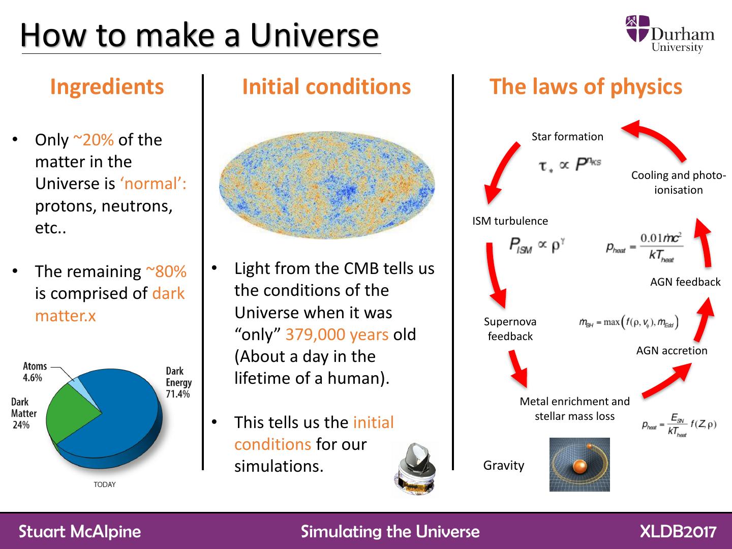
3 .How to make a Universe Ingredients Initial conditions The laws of physics • Only ~20% of the Star formation matter in the Cooling and photo- Universe is ‘normal’: ionisation protons, neutrons, ISM turbulence etc.. • The remaining ~80% • Light from the CMB tells us AGN feedback is comprised of dark the conditions of the matter.x Universe when it was Supernova “only” 379,000 years old feedback AGN accretion (About a day in the lifetime of a human). Metal enrichment and stellar mass loss • This tells us the initial conditions for our simulations. Gravity Stuart McAlpine Simulating the Universe XLDB2017 

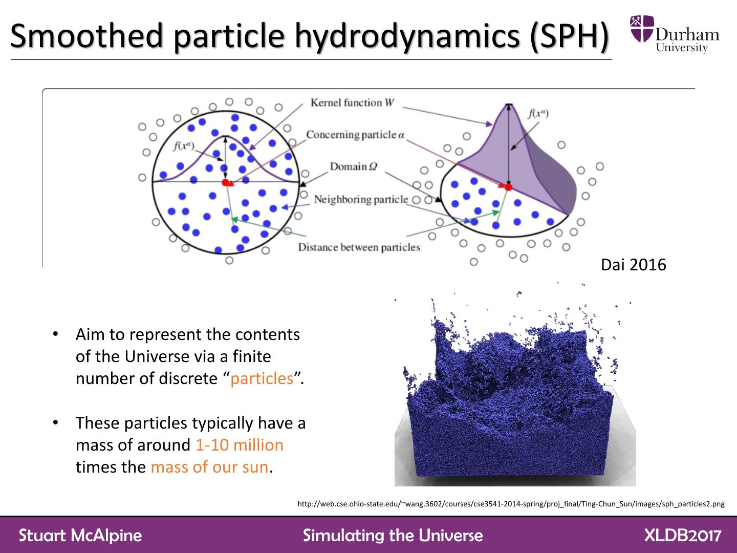
4 .Smoothed particle hydrodynamics (SPH) Dai 2016 • Aim to represent the contents of the Universe via a finite number of discrete “particles”. • These particles typically have a mass of around 1-10 million times the mass of our sun. http://web.cse.ohio-state.edu/~wang.3602/courses/cse3541-2014-spring/proj_final/Ting-Chun_Sun/images/sph_particles2.png Stuart McAlpine Simulating the Universe XLDB2017 

5 .The EAGLE simulation Stuart McAlpine Simulating the Universe XLDB2017 

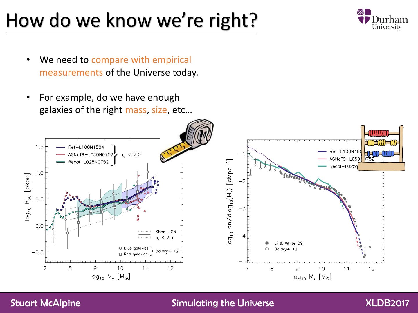
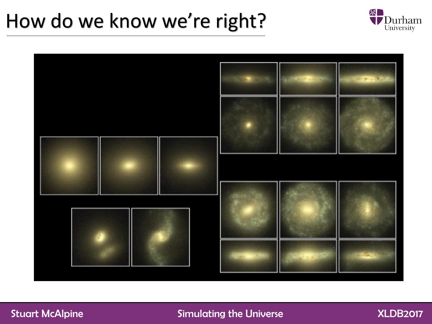
6 .How do we know we’re right? • We need to compare with empirical measurements of the Universe today. • For example, do we have enough galaxies of the right mass, size, etc… Stuart McAlpine Simulating the Universe XLDB2017 

7 .How do we know we’re right? Stuart McAlpine Simulating the Universe XLDB2017 

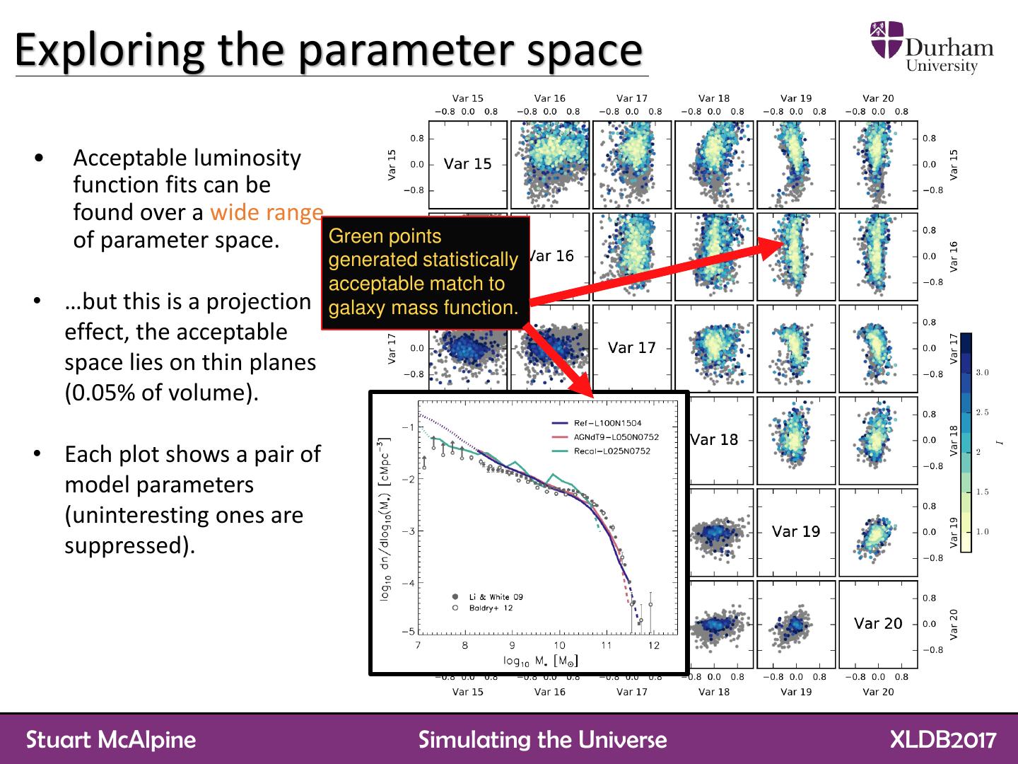
8 .Exploring the parameter space • Acceptable luminosity function fits can be found over a wide range of parameter space. Green points generated statistically acceptable match to • …but this is a projection galaxy mass function. effect, the acceptable space lies on thin planes (0.05% of volume). • Each plot shows a pair of model parameters (uninteresting ones are suppressed). Stuart McAlpine Simulating the Universe XLDB2017 

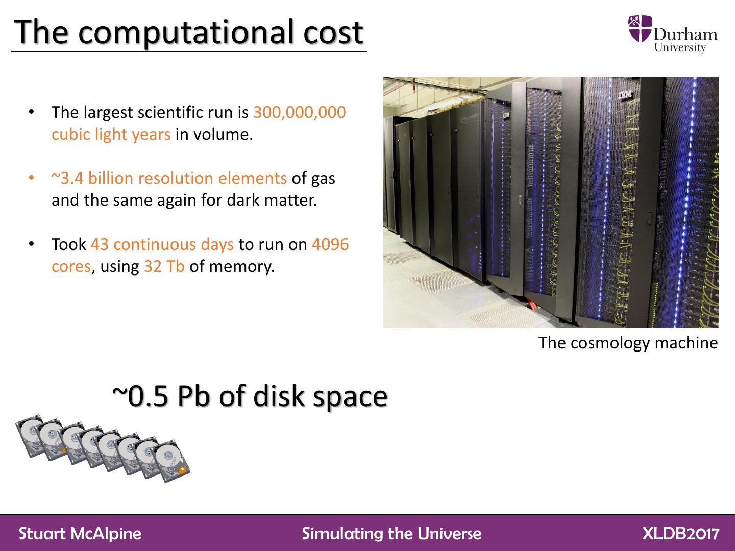
9 .The computational cost • The largest scientific run is 300,000,000 cubic light years in volume. • ~3.4 billion resolution elements of gas and the same again for dark matter. • Took 43 continuous days to run on 4096 cores, using 32 Tb of memory. The cosmology machine ~0.5 Pb of disk space Stuart McAlpine Simulating the Universe XLDB2017 

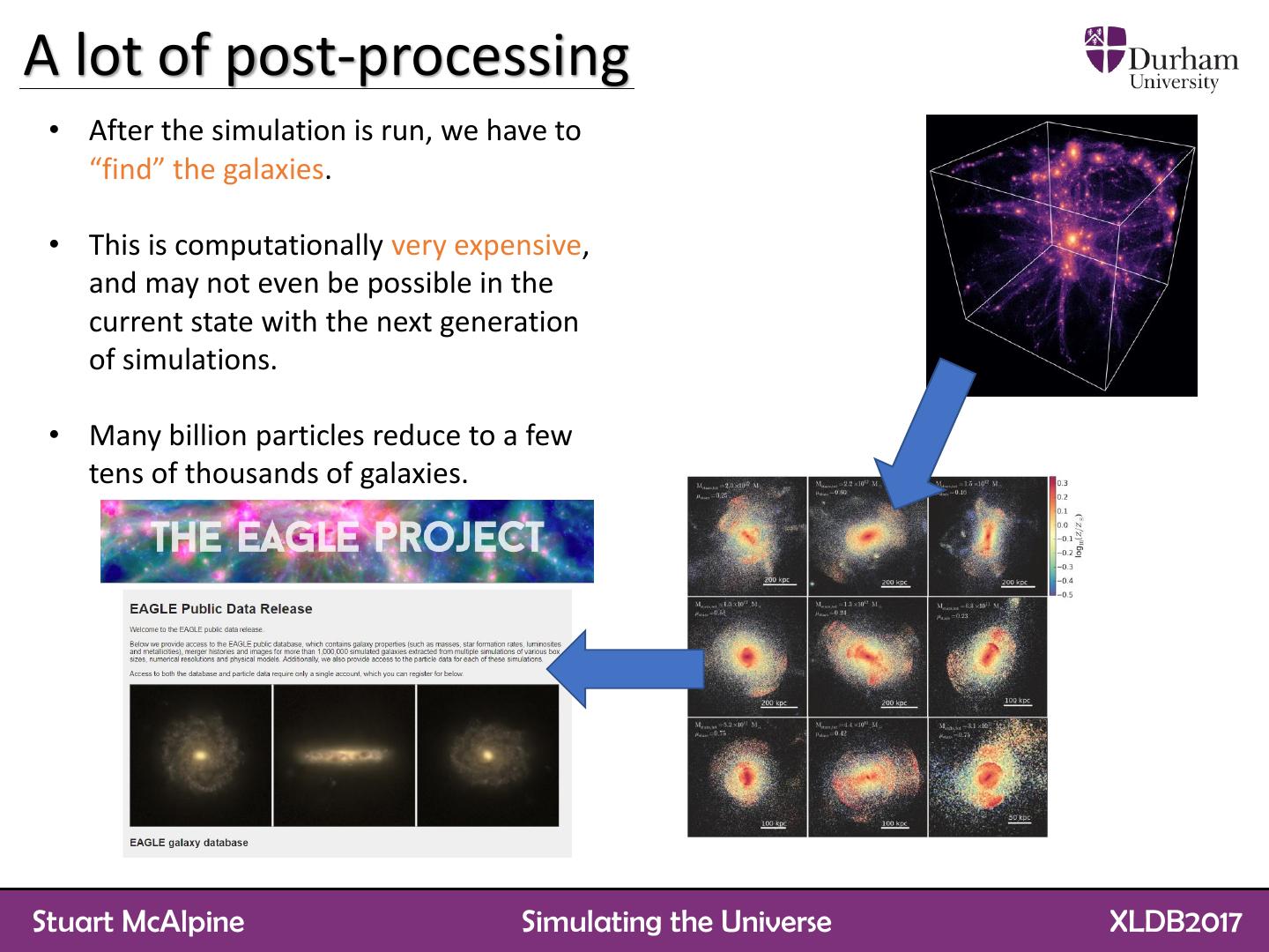
10 .A lot of post-processing • After the simulation is run, we have to “find” the galaxies. • This is computationally very expensive, and may not even be possible in the current state with the next generation of simulations. • Many billion particles reduce to a few tens of thousands of galaxies. Stuart McAlpine Simulating the Universe XLDB2017 

11 . What’s next? Stuart McAlpine Simulating the Universe XLDB2017 

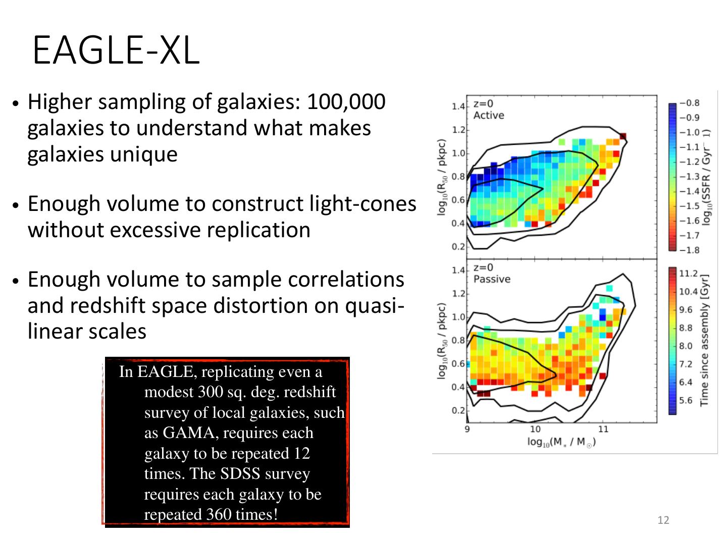
12 . EAGLE-XL • Higher sampling of galaxies: 100,000 galaxies to understand what makes galaxies unique • Enough volume to construct light-cones without excessive replication • Enough volume to sample correlations and redshift space distortion on quasi- linear scales In EAGLE, replicating even a modest 300 sq. deg. redshift survey of local galaxies, such as GAMA, requires each galaxy to be repeated 12 times. The SDSS survey requires each galaxy to be repeated 360 times! 12 

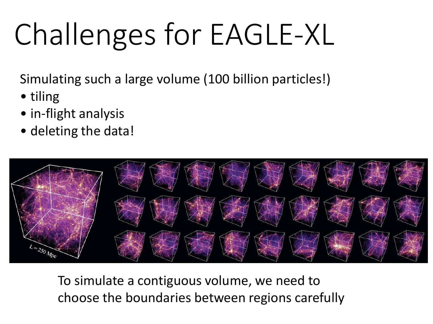
13 .Challenges for EAGLE-XL Simulating such a large volume (100 billion particles!) • tiling • in-flight analysis • deleting the data! To simulate a contiguous volume, we need to choose the boundaries between regions carefully 

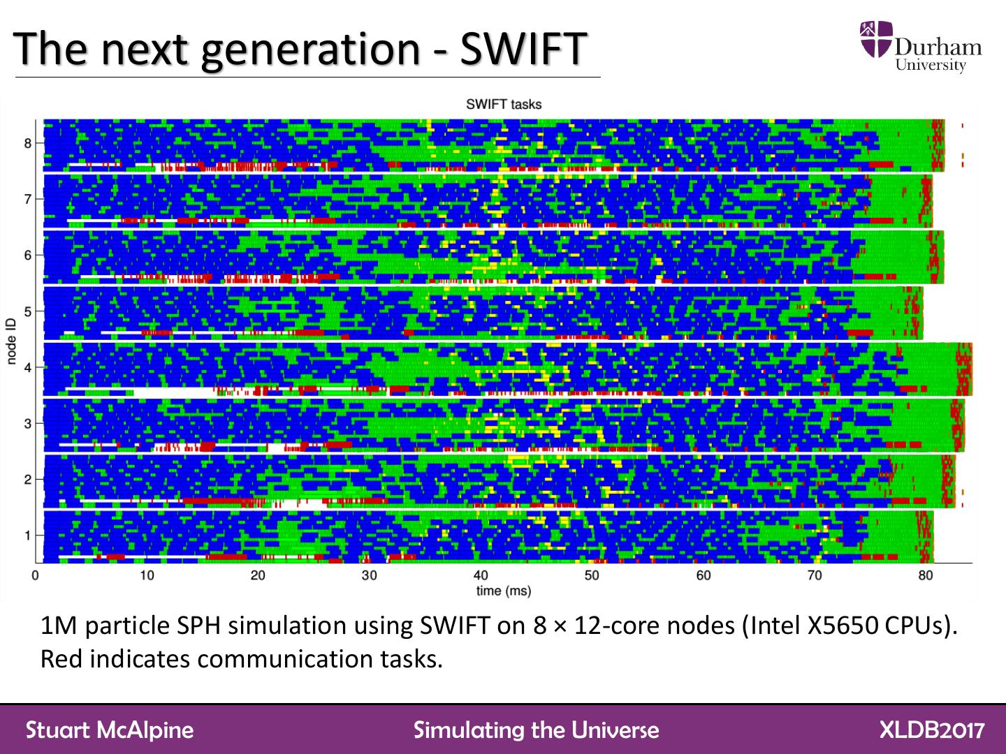
14 .The next generation - SWIFT 1M particle SPH simulation using SWIFT on 8 × 12-core nodes (Intel X5650 CPUs). Red indicates communication tasks. Stuart McAlpine Simulating the Universe XLDB2017 

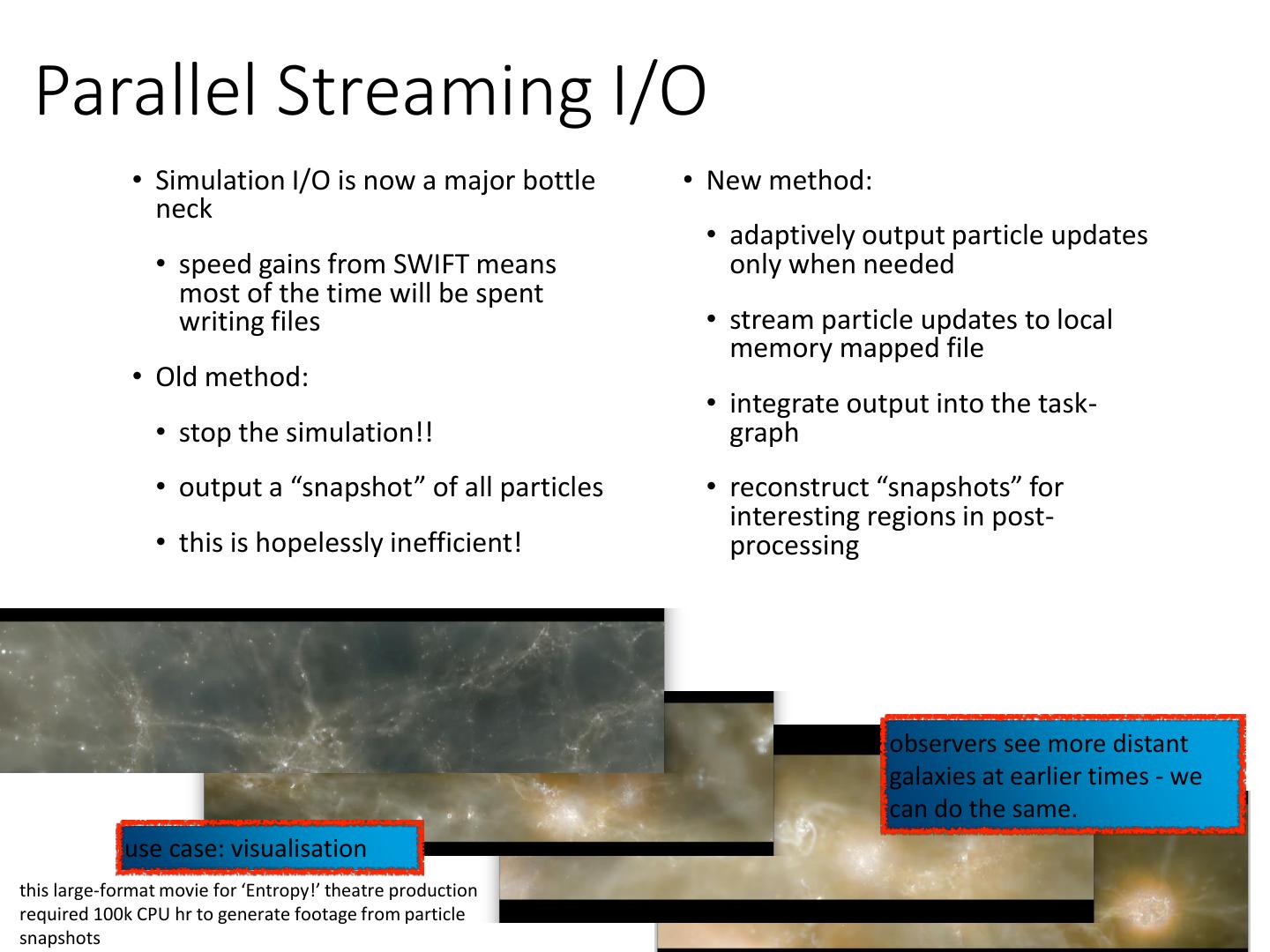
15 . Parallel Streaming I/O • Simulation I/O is now a major bottle • New method: neck • adaptively output particle updates • speed gains from SWIFT means only when needed most of the time will be spent writing files • stream particle updates to local memory mapped file • Old method: • integrate output into the task- • stop the simulation!! graph • output a “snapshot” of all particles • reconstruct “snapshots” for interesting regions in post- • this is hopelessly inefficient! processing observers see more distant galaxies at earlier times - we can do the same. use case: visualisation this large-format movie for ‘Entropy!’ theatre production required 100k CPU hr to generate footage from particle snapshots