036-Fast Obstable Avoidence For Mobile Robots

1 . © 1991 IEEE. Reprinted with permission, from IEEE Journal of Robotics and Automation Vol 7, No 3, June 1991, pp. 278-288. THE VECTOR FIELD HISTOGRAM - FAST OBSTACLE AVOIDANCE FOR MOBILE ROBOTS by J. Borenstein, Member, IEEE and Y. Koren, Senior Member, IEEE The University of Michigan, Ann Arbor Advanced Technology Laboratories 1101 Beal Avenue, Ann Arbor, MI 48109 ABSTRACT A new real-time obstacle avoidance method for mobile robots has been developed and implemented. This method, named the vector field histogram(VFH), permits the detection of unknown obstacles and avoids collisions while simultaneously steering the mobile robot toward the target. The VFH method uses a two-dimensional Cartesian histogram grid as a world model. This world model is updated continuously with range data sampled by on-board range sensors. The VFH method subsequently employs a two-stage data-reduction process in order to compute the desired control commands for the vehicle. In the first stage the histogram grid is reduced to a one- dimensional polar histogram that is constructed around the robot's momentary location. Each sector in the polar histogram contains a value representing the polar obstacle densityin that direction. In the second stage, the algorithm selects the most suitable sector from among all polar histogram sectors with a low polar obstacle density, and the steering of the robot is aligned with that direction. Experimental results from a mobile robot traversing densely cluttered obstacle courses in smooth and continuous motion and at an average speed of 0.6 0.7m/sec demonstrate the power of the VFH method. This work was sponsored by the Department of Energy Grant DE-FG02-86NE37969 

2 . 1. INTRODUCTION Obstacle avoidance is one of the key issues to successful applications of mobile robot systems. All mobile robots feature some kind of collision avoidance, ranging from primitive algorithms that detect an obstacle and stop the robot short of it in order to avoid a collision, through sophisticated algorithms, that enable the robot to detour obstacles. The latter algorithms are much more complex, since they involve not only the detection of an obstacle, but also some kind of quantitative measurements concerning the dimensions of the obstacle. Once these have been determined, the obstacle avoidance algorithm needs to steer the robot around the obstacle and proceed toward the original target. Usually, this procedure requires the robot to stop in front of the obstacle, take the measurements, and only then resume motion. Obstacle avoidance (also called reflexive obstacle avoidance or local path planning) may result in non-optimal paths [5], since no prior knowledge about the environment is used. A brief survey of relevant earlier obstacle avoidance methods is presented in Section 2, while Section 3 summarizes the virtual force field (VFF), an obstacle avoidance method developed earlier by our group at the University of Michigan [5]). While the VFF method provides superior real-time obstacle avoidance for fast mobile robots, some limitations concerning fast travel among densely cluttered obstacles were identified in the course of our experimental work [18]. To overcome these limitations, we developed a new method, named vector field histogram(VFH), which is introduced in Section 4. The VFH method eliminates the shortcomings of the VFF method, yet retains all advantages of its predecessor (as will be shown in Section 4). A comparison of the VFH method to earlier methods is given in Section 5, and Section 6 presents experimental results obtained with our VFH-controlled mobile robot. 2. SURVEY OF EARLIER OBSTACLE AVOIDANCE METHODS This section summarizes relevant obstacle avoidance methods, namely edge-detection, certainty grids, and potential field methods. 2.1 Edge-Detection Methods One popular obstacle avoidance method is based on edge-detection. In this method, an algorithm tries to determine the position of the vertical edges of the obstacle and then steer the robot around either one of the "visible" edges. The line connecting two visible edges is considered to represent one of the boundaries of the obstacle. This method was used in our very early research [4], as well as in several other works [11,21,22,28], all using ultrasonic sensors for obstacle detection. A disadvantage with current implementations of this method is that the robot stops in front of obstacles to gather sensor information. However, this is not an Page 2 

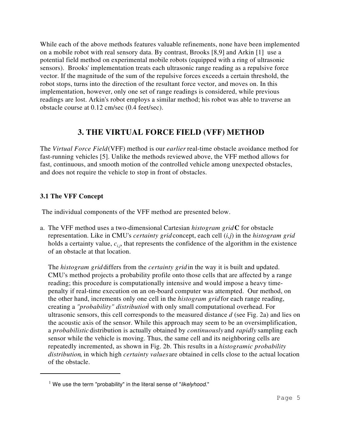
3 .inherent limitation of edge-detection methods; it may be possible to overcome this problem with faster computers in future implementations. In another edge-detection approach (using ultrasonic sensors), the robot remains stationary while taking a panoramic scan of its environment [13,14]. After the application of certain line-fitting algorithms, an edge-based global path planner is instituted to plan the robot's subsequent path. A common drawback of both edge-detection approaches is their sensitivity to sensor accuracy. Ultrasonic sensors present many shortcomings in this respect: Poor directionality limits the accuracy in determining the spatial position of an edge to 10- 50 cm, depending on the distance to the obstacle and the angle between the obstacle surface and the acoustic axis. Frequent misreadings are caused by either ultrasonic noise from external sources or stray reflections from neighboring sensors (i.e., crosstalk). Misreadings cannot always be filtered out and they cause the algorithm to falsely detect edges. Specular reflections occur when the angle between the wavefront and the normal to a smooth surface is too large. In this case the surface reflects the incoming ultra-sound waves away from the sensor, and the obstacle is either not detected, or "seen" as much smaller than it is in reality (since only part of the surface is detected). Any one of these errors can cause the algorithm to determine the existence of an edge at a completely wrong location, oftentimes resulting in highly unlikely paths. 2.2 The Certainty Grid for Obstacle Representation A method for probabilistic representation of obstacles in a grid-type world model has been developed at Carnegie-Mellon University (CMU) [13,23,24]. This world model, called certainty grid, is especially suited to the accommodation of inaccurate sensor data such as range measurements from ultrasonic sensors. In the certainty grid, the robot's work area is represented by a two-dimensional array of square elements, denoted as cells. Each cell contains a certainty value (CV) that indicates the measure of confidence that an obstacle exists within the cell area. With the CMU method, CVs are updated by a probability function that takes into account the characteristics of a given sensor. Ultrasonic sensors, for example, have a conical field of view. A typical ultrasonic sensor [25] returns a radial measure of the distance to the nearest object within the cone, yet does not specify the angular location of the object. (Fig. 1 shows the area A in which an object must be located in order to result in a distance measurement d). If an object is detected Page 3 

4 .by an ultrasonic sensor, it is more likely that this object is closer to the acoustic axis of the sensor than to the periphery of the conical field of view [4]. For this reason, CMU's probabilistic function Cx increases CVs in cells close to the acoustic axis more than CVs in cells at the periphery. In CMU's applications of this method [23,24], the mobile robot remains stationary while it takes a panoramic scan with its 24 ultrasonic sensors. Next, the probabilistic function Cx is applied to each of the 24 range readings, updating the Object certainty grid. Finally, the robot moves to a new location, stops, and repeats the procedure. After the robot traverses a room in this manner, the resulting certainty grid represents a fairly accurate map of the room. A global path-planning method is then employed for off-line calculations of subsequent robot paths. 2.3 Potential Field Methods The idea of imaginary forces acting on a robot has been suggested by Khatib [16]. In this method, obstacles exert repulsive vfh05.ds4, p18fig2.wmf forces, while the target applies an Figure. 1: Two-dimensional projection of the conical attractive force to the robot. A resultant field of view of an ultrasonic sensor. A range reading d force vector R, comprising the sum of a indicates the existence of an object somewhere within the shaded region A (Carnegie Mellon's method). target-directed attractive force and repulsive forces from obstacles, is calculated for a given robot position. With R as the accelerating force acting on the robot, the robot's new position for a given time interval is calculated, and the algorithm is repeated. Krogh [19] has enhanced this concept further by taking into consideration the robot's velocity in the vicinity of obstacles. Thorpe [27] has applied the potential field method to off-line path planning and Krogh and Thorpe [20] suggest a combined method for global and local path planning, which uses a "Generalized Potential Field" approach. Newman and Hogan [15] introduce the construction of potential functions through combining individual obstacle functions with logical operations. Common to these methods is the assumption of a known and prescribed world model, in which simple, predefined geometric shapes represent obstacles and the robot's path is gen- erated off-line. Page 4 

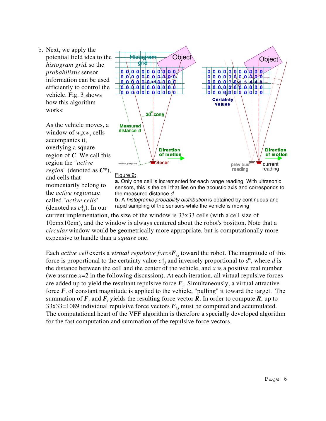
5 .While each of the above methods features valuable refinements, none have been implemented on a mobile robot with real sensory data. By contrast, Brooks [8,9] and Arkin [1] use a potential field method on experimental mobile robots (equipped with a ring of ultrasonic sensors). Brooks' implementation treats each ultrasonic range reading as a repulsive force vector. If the magnitude of the sum of the repulsive forces exceeds a certain threshold, the robot stops, turns into the direction of the resultant force vector, and moves on. In this implementation, however, only one set of range readings is considered, while previous readings are lost. Arkin's robot employs a similar method; his robot was able to traverse an obstacle course at 0.12 cm/sec (0.4 feet/sec). 3. THE VIRTUAL FORCE FIELD (VFF) METHOD The Virtual Force Field (VFF) method is our earlier real-time obstacle avoidance method for fast-running vehicles [5]. Unlike the methods reviewed above, the VFF method allows for fast, continuous, and smooth motion of the controlled vehicle among unexpected obstacles, and does not require the vehicle to stop in front of obstacles. 3.1 The VFF Concept The individual components of the VFF method are presented below. a. The VFF method uses a two-dimensional Cartesian histogram grid C for obstacle representation. Like in CMU's certainty grid concept, each cell (i,j) in the histogram grid holds a certainty value, ci,j, that represents the confidence of the algorithm in the existence of an obstacle at that location. The histogram grid differs from the certainty grid in the way it is built and updated. CMU's method projects a probability profile onto those cells that are affected by a range reading; this procedure is computationally intensive and would impose a heavy time- penalty if real-time execution on an on-board computer was attempted. Our method, on the other hand, increments only one cell in the histogram grid for each range reading, creating a "probability" distribution1 with only small computational overhead. For ultrasonic sensors, this cell corresponds to the measured distance d (see Fig. 2a) and lies on the acoustic axis of the sensor. While this approach may seem to be an oversimplification, a probabilistic distribution is actually obtained by continuously and rapidly sampling each sensor while the vehicle is moving. Thus, the same cell and its neighboring cells are repeatedly incremented, as shown in Fig. 2b. This results in a histogramic probability distribution, in which high certainty values are obtained in cells close to the actual location of the obstacle. 1 We use the term "probability" in the literal sense of "likelyhood." Page 5 

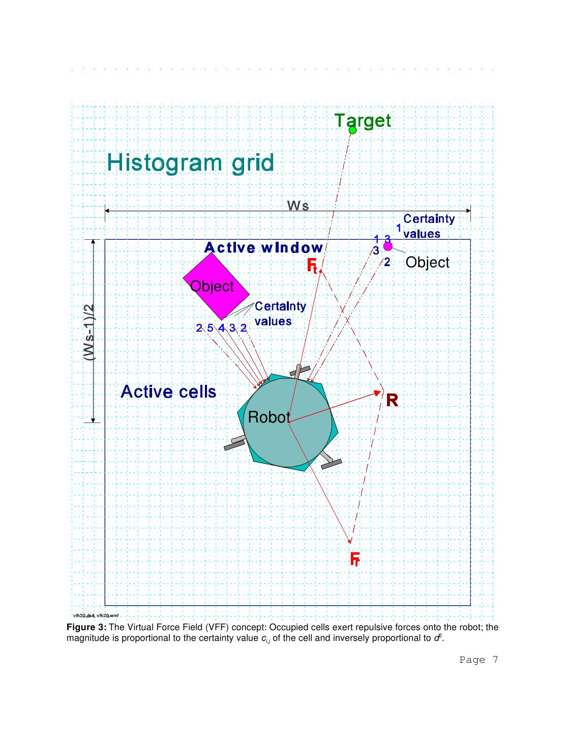
6 .b. Next, we apply the potential field idea to the Object Object histogram grid, so the probabilistic sensor information can be used efficiently to control the vehicle. Fig. 3 shows how this algorithm works: As the vehicle moves, a window of wsxws cells accompanies it, overlying a square region of C. We call this region the "active vfh10.ds4, p18fig3.wmf current region" (denoted as C*), reading Figure 2: and cells that a. Only one cell is incremented for each range reading. With ultrasonic momentarily belong to sensors, this is the cell that lies on the acoustic axis and corresponds to the active region are the measured distance d. called "active cells" b. A histogramic probability distribution is obtained by continuous and (denoted as c*i,j). In our rapid sampling of the sensors while the vehicle is moving current implementation, the size of the window is 33x33 cells (with a cell size of 10cmx10cm), and the window is always centered about the robot's position. Note that a circular window would be geometrically more appropriate, but is computationally more expensive to handle than a square one. Each active cell exerts a virtual repulsive forceFi,j toward the robot. The magnitude of this force is proportional to the certainty value c*i,j and inversely proportional to dx, where d is the distance between the cell and the center of the vehicle, and x is a positive real number (we assume x=2 in the following discussion). At each iteration, all virtual repulsive forces are added up to yield the resultant repulsive force Fr. Simultaneously, a virtual attractive force Ft of constant magnitude is applied to the vehicle, "pulling" it toward the target. The summation of Fr and Ft yields the resulting force vector R. In order to compute R, up to 33x33=1089 individual repulsive force vectors Fi,j must be computed and accumulated. The computational heart of the VFF algorithm is therefore a specially developed algorithm for the fast computation and summation of the repulsive force vectors. Page 6 

7 . Object Object Robot Figure 3: The Virtual Force Field (VFF) concept: Occupied cells exert repulsive forces onto the robot; the magnitude is proportional to the certainty value ci,j of the cell and inversely proportional to d2. Page 7 

8 .c. Combining the above two concepts (a.) and (b.) in real-time enables sensor data to influence the steering control immediately. In practice, each range reading is recorded into the histogram grid as soon as it becomes available, and the subsequent calculation of R takes this data-point into account. This feature gives the vehicle fast response to obstacles that appear suddenly, resulting in fast reflexive behavior imperative at high speeds. 3.2 Shortcomings of the VFF Method The VFF method has been implemented and extensively tested on-board a mobile robot equipped with a ring of 24 ultrasonic sensors (see Section 6). Under most conditions, the VFF-controlled robot performed very well. Typically, it traversed an obstacle course at an average speed of 0.5m/sec, provided the obstacles were placed at least 1.8m apart (the robot diameter is 0.8m). With less clearance between two obstacles (e.g., a doorway), some problems were encountered. Sometimes, the robot would not pass through a doorway, because the repulsive forces from both sides of the doorway resulted in a force that pushed the robot away. Another problem arose out of the discrete nature of the histogram grid. In order to efficiently calculate repulsive forces in real-time, the robot's momentary position is mapped onto the histogram grid. Whenever this position changes from one cell to another, drastic changes in the resultant R may be encountered. The following numeric example explains this point. Consider a repulsive force generated by a cell (m,n) and applied to the robot's momentary position at (m,n+6), which is six cells away (i.e., 0.6 m, with a cell size of 10x10cm). The magnitude of this particular force vector is |Fm,n|=k/0.62=2.8k. As the robot advances by one cell, and its position corresponds to cell (m,n+5), the new force vector is |F'm,n|=k/0.52=4k. The change is 42%. Changes of this magnitude cause considerable fluctuations in the steering control. The situation is even worse when the magnitude of the target-directed constant attractive force Ft lies between the directions of the two successive forces |F| and |F'| (this condition is in fact most likely, because it corresponds to the "steady state" condition when the robot travels alongside an obstacle). In this situation, the direction of the resultant R may fluctuate by up to 180o. For this reason it is necessary to smooth the control signal to the steer- ing motor by adding a low-pass filter to the VFF control loop [5]. This filter, however, intro- duces a delay that adversely affects the robot's steering response to unexpected obstacles. Finally, we also identified a problem that occurs when the robot travels in narrow corridors. When traveling along the center-line between the two corridor walls, the robot's motion is stable. If, however, the robot strays slightly to either side of the center-line, it experiences a strong virtual repulsive force from the closer wall. This force usually "pushes" the robot across the center-line, and the process repeats with the other wall. Under certain conditions, this process results in oscillatory and unstable motion [17,18]. Page 8 

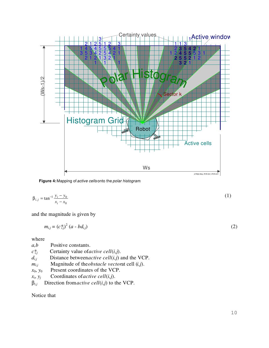
9 . 4. THE VECTOR FIELD HISTOGRAM (VFH) METHOD Careful analysis of the shortcomings of the VFF method reveals its inherent problem: excessively drastic data reduction that occurs when the individual repulsive forces from histogram grid cells are added up to calculate the resultant force vector Fr. Hundreds of data points are reduced in one step to only two items: direction and magnitude of Fr. Consequently, detailed information about the local obstacle distribution is lost. To remedy this shortcoming, we have developed a new method called the vector field histogram (VFH). The VFH method employs a two-stage data reductiontechnique, rather than the single-step technique used by the VFF method. Thus, three levels of data representation exist: a. The highest level holds the detailed description of the robot's environment. In this level, the two-dimensional Cartesian histogram grid C is continuously updated in real-time with range data sampled by the on-board range sensors. This process is identical to the one described in Section 3 for the VFF method. b. At the intermediate level, a one-dimensional polar histogram H is constructed around the robot's momentary location. H comprises n angular sectors of width α. A transformation (described in Section 4.1, below) maps the active region C* onto H, resulting in each sector k holding a value hk that represents the polar obstacle densityin the direction that corresponds to sector k. c. The lowest level of data representation is the output of the VFH algorithm: the reference values for the drive and steer controllers of the vehicle. The following sections describe the two data reduction stages in more detail. 4.1 First Data Reduction and Creation of the Polar Histogram The first data-reduction stage maps the active region C* of the histogram grid C onto the polar histogram H, as follows: As with our earlier VFF method, a window moves with the vehicle, overlying a square region of wsxws cells in the histogram grid (see Fig. 4). The contents of each active cell in the histogram grid are now treated as an obstacle vector, the direction of which is determined by the direction β from the cell to the Vehicle Center Point (VCP)2 2 For symmetrically shaped vehicles, the VCP is easily defined as the geometric center of the vehicle. For rectangular vehicles, it is possible to chose two VCPs, e.g., one each at the center-point of the front and rear axles. Page 9 

10 . Certainty values 3 1Active window 2 1 2 5 1 2 3 1 1 3 1 4 5 4 5 5 54 1 2 3 5 421 3 5 3 4 2 5 42 1 12 4 5 553 1 2 1 2 1 3 21 2 5 5 212 1 1 1 3 2 1 lar Histogram Po (Ws-1)/2 Sector k Histogram Grid Robot VCP Active cells Ws p16fig4.dwg, vfh30.ds4, vfh30.wmf Figure 4: Mapping of active cells onto the polar histogram. y i − y0 (1) β i , j = tan −1 xi − x0 and the magnitude is given by mi,j = (c*i,j)2 (a - bdi,j) (2) where a,b Positive constants. c*i,j Certainty value of active cell (i,j). di,j Distance between active cell (i,j) and the VCP. mi,j Magnitude of the obstacle vectorat cell (i,j). x0, y0 Present coordinates of the VCP. xi, yj Coordinates of active cell (i,j). βi,j Direction from active cell (i,j) to the VCP. Notice that 10 

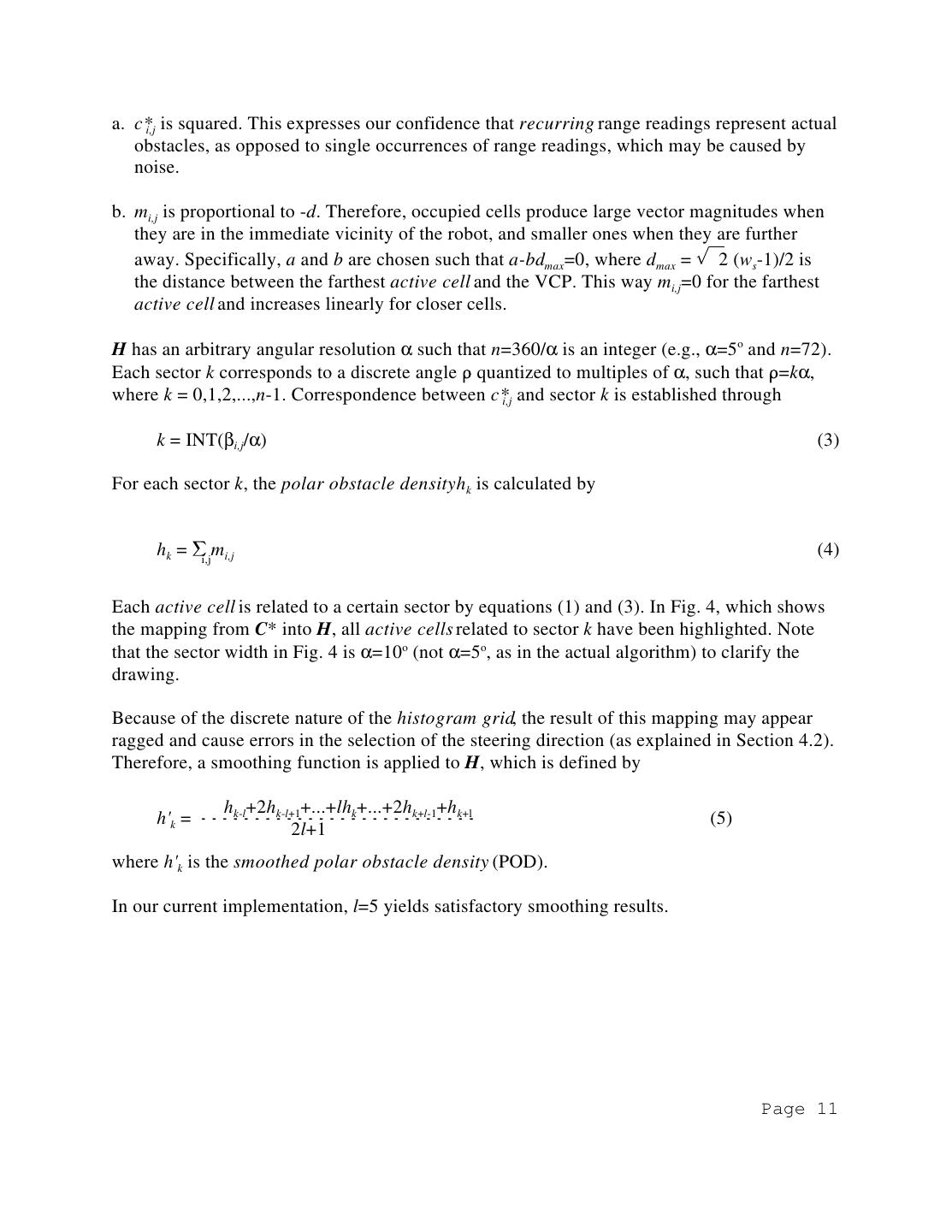
11 .a. c*i,j is squared. This expresses our confidence that recurring range readings represent actual obstacles, as opposed to single occurrences of range readings, which may be caused by noise. b. mi,j is proportional to -d. Therefore, occupied cells produce large vector magnitudes when they are in the immediate vicinity of the robot, and smaller ones when they are further away. Specifically, a and b are chosen such that a-bdmax=0, where dmax = 2 (ws-1)/2 is the distance between the farthest active cell and the VCP. This way mi,j=0 for the farthest active cell and increases linearly for closer cells. H has an arbitrary angular resolution α such that n=360/α is an integer (e.g., α=5o and n=72). Each sector k corresponds to a discrete angle quantized to multiples of α, such that =kα, where k = 0,1,2,...,n-1. Correspondence between c*i,j and sector k is established through k = INT(βi,j/α) (3) For each sector k, the polar obstacle densityhk is calculated by hk = mi,j i,j (4) Each active cell is related to a certain sector by equations (1) and (3). In Fig. 4, which shows the mapping from C* into H, all active cells related to sector k have been highlighted. Note that the sector width in Fig. 4 is α=10o (not α=5o, as in the actual algorithm) to clarify the drawing. Because of the discrete nature of the histogram grid, the result of this mapping may appear ragged and cause errors in the selection of the steering direction (as explained in Section 4.2). Therefore, a smoothing function is applied to H, which is defined by hk-l+2hk-l+1+...+lhk+...+2hk+l-1+hk+l h'k = -------------------------- (5) 2l+1 where h'k is the smoothed polar obstacle density (POD). In our current implementation, l=5 yields satisfactory smoothing results. Page 11 

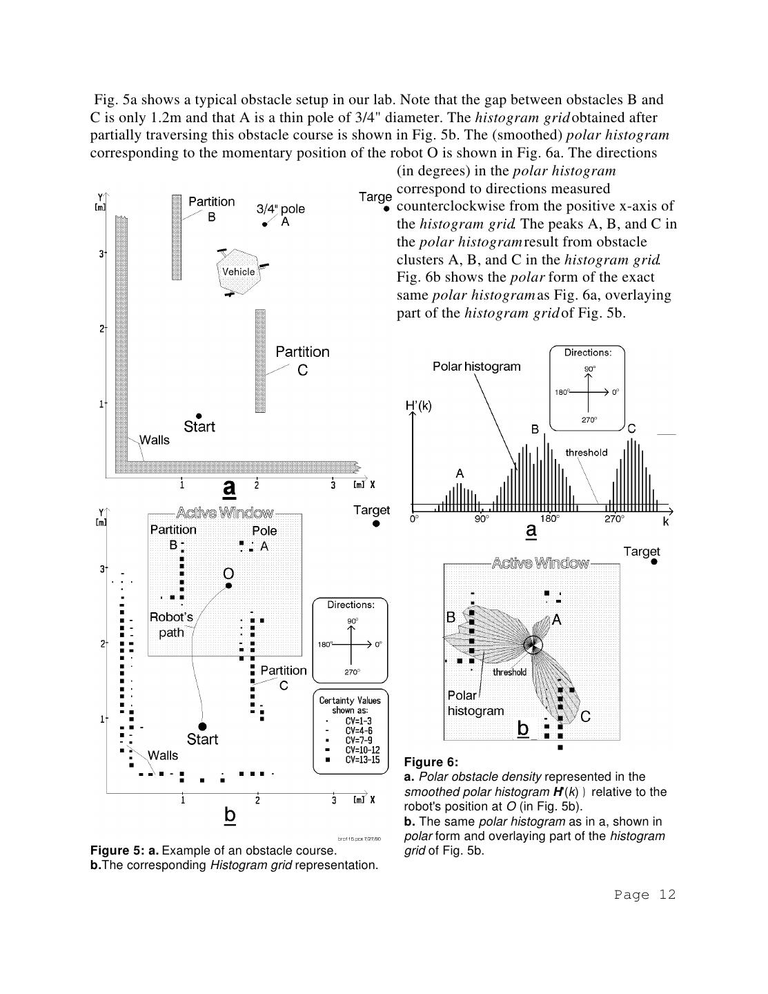
12 . Fig. 5a shows a typical obstacle setup in our lab. Note that the gap between obstacles B and C is only 1.2m and that A is a thin pole of 3/4" diameter. The histogram grid obtained after partially traversing this obstacle course is shown in Fig. 5b. The (smoothed) polar histogram corresponding to the momentary position of the robot O is shown in Fig. 6a. The directions (in degrees) in the polar histogram correspond to directions measured counterclockwise from the positive x-axis of the histogram grid. The peaks A, B, and C in the polar histogram result from obstacle clusters A, B, and C in the histogram grid. Fig. 6b shows the polar form of the exact same polar histogram as Fig. 6a, overlaying part of the histogram grid of Fig. 5b. Figure 6: a. Polar obstacle density represented in the smoothed polar histogram H'(k) ) relative to the robot's position at O (in Fig. 5b). b. The same polar histogram as in a, shown in polar form and overlaying part of the histogram Figure 5: a. Example of an obstacle course. grid of Fig. 5b. b.The corresponding Histogram grid representation. Page 12 

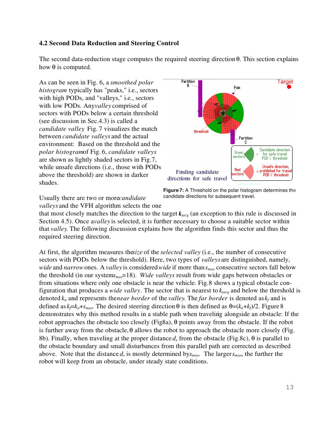
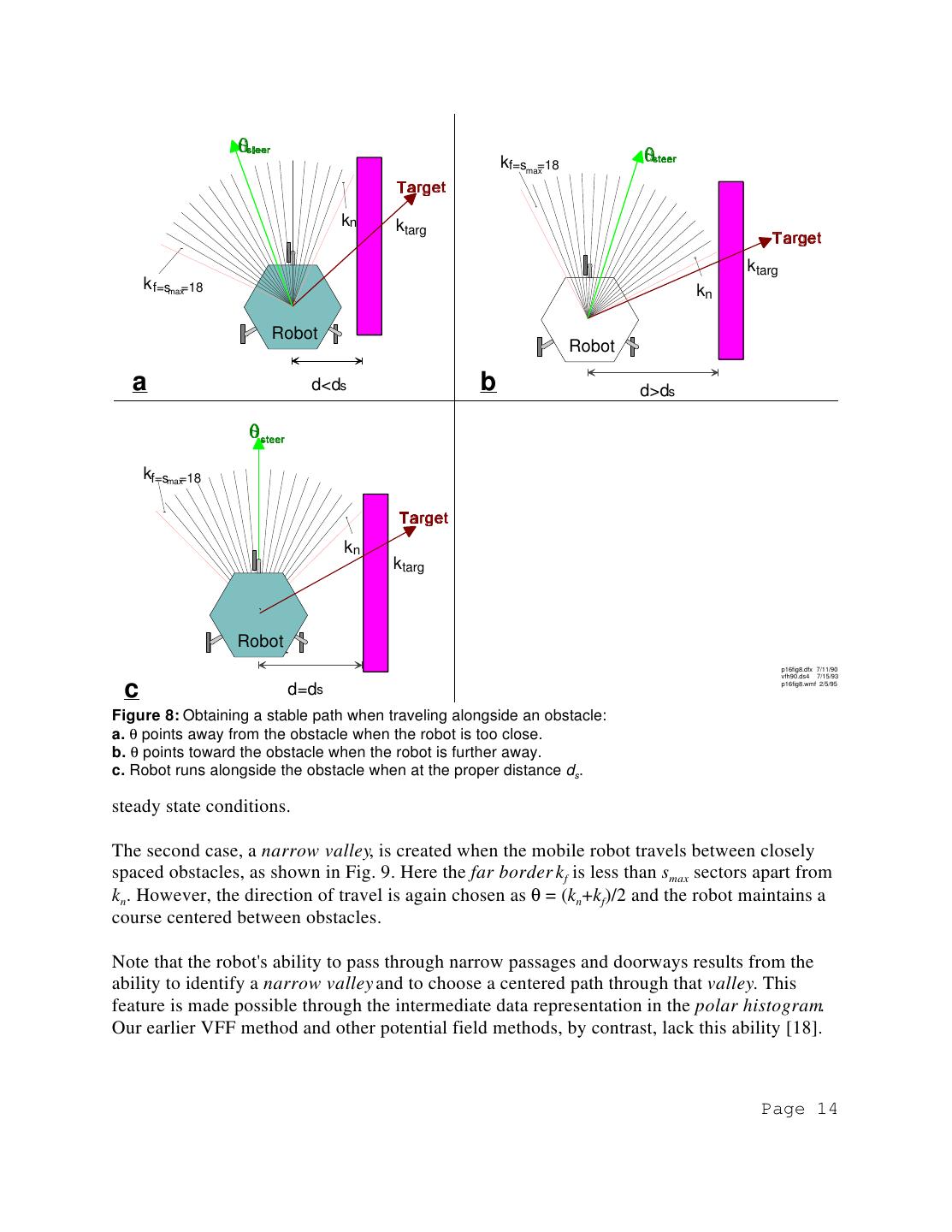
13 .4.2 Second Data Reduction and Steering Control The second data-reduction stage computes the required steering direction θ. This section explains how θ is computed. As can be seen in Fig. 6, a smoothed polar histogram typically has "peaks," i.e., sectors with high PODs, and "valleys," i.e., sectors with low PODs. Anyvalley comprised of sectors with PODs below a certain threshold (see discussion in Sec.4.3) is called a candidate valley. Fig. 7 visualizes the match between candidate valleys and the actual environment: Based on the threshold and the polar histogramof Fig. 6, candidate valleys are shown as lightly shaded sectors in Fig.7, while unsafe directions (i.e., those with PODs above the threshold) are shown in darker shades. Figure 7: A Threshold on the polar histogram determines the Usually there are two or morecandidate candidate directions for subsequent travel. valleys and the VFH algorithm selects the one that most closely matches the direction to the target kt targ (an exception to this rule is discussed in Section 4.5). Once avalley is selected, it is further necessary to choose a suitable sector within that valley. The following discussion explains how the algorithm finds this sector and thus the required steering direction. At first, the algorithm measures thesize of the selected valley (i.e., the number of consecutive sectors with PODs below the threshold). Here, two types of valleys are distinguished, namely, wide and narrow ones. A valley is considered wide if more than smax consecutive sectors fall below the threshold (in our systemsmax=18). Wide valleys result from wide gaps between obstacles or from situations where only one obstacle is near the vehicle. Fig. 8 shows a typical obstacle con- figuration that produces a wide valley. The sector that is nearest to ktarg and below the threshold is denoted kn and represents the near border of the valley. The far border is denoted as kf and is defined as kf=kn+smax. The desired steering direction θ is then defined as θ=(kn+kf)/2. Figure 8 demonstrates why this method results in a stable path when traveling i alongside an obstacle: If the robot approaches the obstacle too closely (Fig.8a), θ points away from the obstacle. If the robot is further away from the obstacle, θ allows the robot to approach the obstacle more closely (Fig. 8b). Finally, when traveling at the proper distance ds from the obstacle (Fig.8c), θ is parallel to the obstacle boundary and small disturbances from this parallel path are corrected as described above. Note that the distance ds is mostly determined bysmax. The larger smax, the further the robot will keep from an obstacle, under steady state conditions. 13 

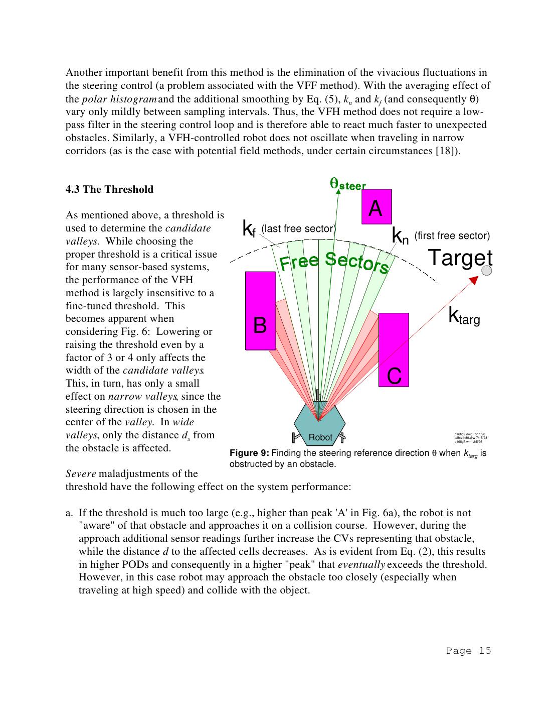
14 . kf=smax=18 kn ktarg ktarg k f=smax=18 kn Robot Robot a d<ds b d>ds kf=smax=18 kn ktarg Robot Robot p16fig8.dfx 7/11/90 vfh90.ds4 7/15/93 c d=ds p16fig8.wmf 2/5/95 Figure 8: Obtaining a stable path when traveling alongside an obstacle: a. θ points away from the obstacle when the robot is too close. b. θ points toward the obstacle when the robot is further away. c. Robot runs alongside the obstacle when at the proper distance ds. steady state conditions. The second case, a narrow valley, is created when the mobile robot travels between closely spaced obstacles, as shown in Fig. 9. Here the far border kf is less than smax sectors apart from kn. However, the direction of travel is again chosen as θ = (kn+kf)/2 and the robot maintains a course centered between obstacles. Note that the robot's ability to pass through narrow passages and doorways results from the ability to identify a narrow valley and to choose a centered path through that valley. This feature is made possible through the intermediate data representation in the polar histogram. Our earlier VFF method and other potential field methods, by contrast, lack this ability [18]. Page 14 

15 .Another important benefit from this method is the elimination of the vivacious fluctuations in the steering control (a problem associated with the VFF method). With the averaging effect of the polar histogram and the additional smoothing by Eq. (5), kn and kf (and consequently θ) vary only mildly between sampling intervals. Thus, the VFH method does not require a low- pass filter in the steering control loop and is therefore able to react much faster to unexpected obstacles. Similarly, a VFH-controlled robot does not oscillate when traveling in narrow corridors (as is the case with potential field methods, under certain circumstances [18]). 4.3 The Threshold As mentioned above, a threshold is A A used to determine the candidate valleys. While choosing the k f (last free sector) kn (first free sector) proper threshold is a critical issue for many sensor-based systems, Target the performance of the VFH method is largely insensitive to a fine-tuned threshold. This becomes apparent when k targ considering Fig. 6: Lowering or B raising the threshold even by a factor of 3 or 4 only affects the width of the candidate valleys. This, in turn, has only a small C effect on narrow valleys, since the steering direction is chosen in the center of the valley. In wide valleys, only the distance ds from Robot p16fig9.dwg 7/11/90 \vfh\vfh80.drw 7/15/93 p16fig7.wmf 2/5/95 the obstacle is affected. Figure 9: Finding the steering reference direction θ when ktarg is obstructed by an obstacle. Severe maladjustments of the threshold have the following effect on the system performance: a. If the threshold is much too large (e.g., higher than peak 'A' in Fig. 6a), the robot is not "aware" of that obstacle and approaches it on a collision course. However, during the approach additional sensor readings further increase the CVs representing that obstacle, while the distance d to the affected cells decreases. As is evident from Eq. (2), this results in higher PODs and consequently in a higher "peak" that eventually exceeds the threshold. However, in this case robot may approach the obstacle too closely (especially when traveling at high speed) and collide with the object. Page 15 

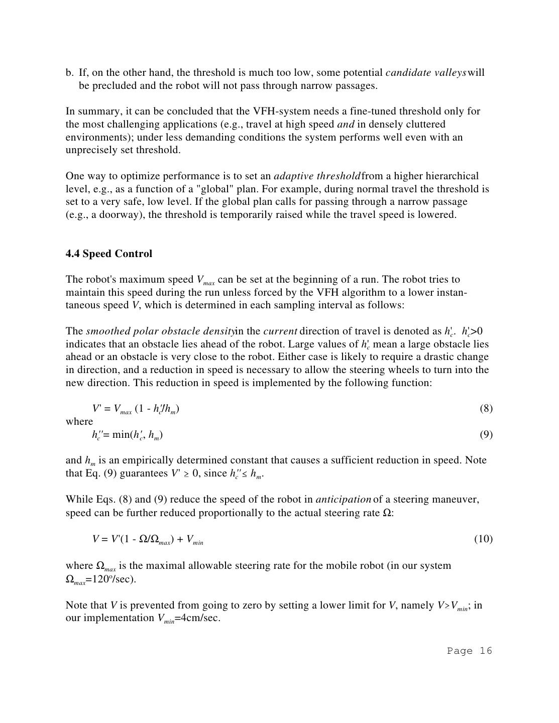
16 .b. If, on the other hand, the threshold is much too low, some potential candidate valleys will be precluded and the robot will not pass through narrow passages. In summary, it can be concluded that the VFH-system needs a fine-tuned threshold only for the most challenging applications (e.g., travel at high speed and in densely cluttered environments); under less demanding conditions the system performs well even with an unprecisely set threshold. One way to optimize performance is to set an adaptive threshold from a higher hierarchical level, e.g., as a function of a "global" plan. For example, during normal travel the threshold is set to a very safe, low level. If the global plan calls for passing through a narrow passage (e.g., a doorway), the threshold is temporarily raised while the travel speed is lowered. 4.4 Speed Control The robot's maximum speed Vmax can be set at the beginning of a run. The robot tries to maintain this speed during the run unless forced by the VFH algorithm to a lower instan- taneous speed V, which is determined in each sampling interval as follows: The smoothed polar obstacle densityin the current direction of travel is denoted as h'. c h'>0 c indicates that an obstacle lies ahead of the robot. Large values of h'c mean a large obstacle lies ahead or an obstacle is very close to the robot. Either case is likely to require a drastic change in direction, and a reduction in speed is necessary to allow the steering wheels to turn into the new direction. This reduction in speed is implemented by the following function: V' = Vmax (1 - h'' c/hm) (8) where h'' c = min(h', c hm) (9) and hm is an empirically determined constant that causes a sufficient reduction in speed. Note that Eq. (9) guarantees V' 0, since h'' c hm. While Eqs. (8) and (9) reduce the speed of the robot in anticipation of a steering maneuver, speed can be further reduced proportionally to the actual steering rate Ω: V = V'(1 - Ω/Ωmax) + Vmin (10) where Ωmax is the maximal allowable steering rate for the mobile robot (in our system Ωmax=120o/sec). Note that V is prevented from going to zero by setting a lower limit for V, namely V Vmin; in our implementation Vmin=4cm/sec. Page 16 

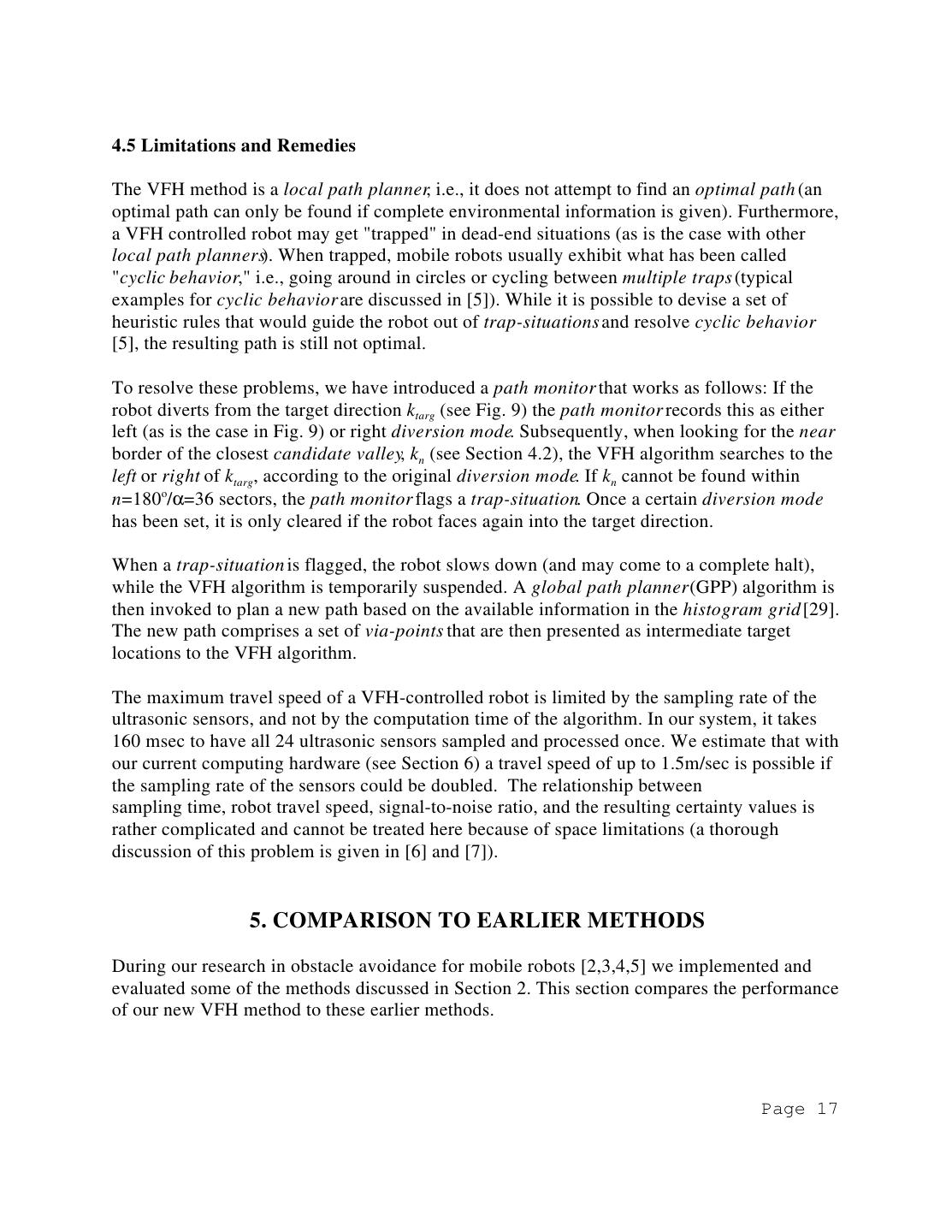
17 .4.5 Limitations and Remedies The VFH method is a local path planner, i.e., it does not attempt to find an optimal path (an optimal path can only be found if complete environmental information is given). Furthermore, a VFH controlled robot may get "trapped" in dead-end situations (as is the case with other local path planners). When trapped, mobile robots usually exhibit what has been called "cyclic behavior," i.e., going around in circles or cycling between multiple traps (typical examples for cyclic behavior are discussed in [5]). While it is possible to devise a set of heuristic rules that would guide the robot out of trap-situations and resolve cyclic behavior [5], the resulting path is still not optimal. To resolve these problems, we have introduced a path monitor that works as follows: If the robot diverts from the target direction ktarg (see Fig. 9) the path monitor records this as either left (as is the case in Fig. 9) or right diversion mode. Subsequently, when looking for the near border of the closest candidate valley, kn (see Section 4.2), the VFH algorithm searches to the left or right of ktarg, according to the original diversion mode. If kn cannot be found within n=180o/α=36 sectors, the path monitor flags a trap-situation. Once a certain diversion mode has been set, it is only cleared if the robot faces again into the target direction. When a trap-situation is flagged, the robot slows down (and may come to a complete halt), while the VFH algorithm is temporarily suspended. A global path planner (GPP) algorithm is then invoked to plan a new path based on the available information in the histogram grid [29]. The new path comprises a set of via-points that are then presented as intermediate target locations to the VFH algorithm. The maximum travel speed of a VFH-controlled robot is limited by the sampling rate of the ultrasonic sensors, and not by the computation time of the algorithm. In our system, it takes 160 msec to have all 24 ultrasonic sensors sampled and processed once. We estimate that with our current computing hardware (see Section 6) a travel speed of up to 1.5m/sec is possible if the sampling rate of the sensors could be doubled. The relationship between sampling time, robot travel speed, signal-to-noise ratio, and the resulting certainty values is rather complicated and cannot be treated here because of space limitations (a thorough discussion of this problem is given in [6] and [7]). 5. COMPARISON TO EARLIER METHODS During our research in obstacle avoidance for mobile robots [2,3,4,5] we implemented and evaluated some of the methods discussed in Section 2. This section compares the performance of our new VFH method to these earlier methods. Page 17 

18 .5.1 Comparison to Edge-Detection Methods The blurry and inaccurate data produced by ultrasonic sensors does not provide the sharply defined contours required by edge-detection methods. Consequently, misreadings or inaccurate range measurements may be interpreted as part of an obstacle, thereby distorting the perceived shape of the obstacle. The VFH method, on the other hand, reacts to clusters of range readings. As soon as a range reading has been sampled, it becomes available to the steering controller (via the histogram grid) and can influence the path of the vehicle immediately. A single range reading will have only minor influence on the path, while repeated range readings in a confined area (cluster) will cause a more drastic change of direction for the vehicle. The force field method developed by Brooks [8,9] and the similar method developed by Arkin [1], do function in experimental real-time systems, using actual sensory data [8,9]. However, these methods are somewhat oversimplified, since a threshold determines if an object is at a safe distance or too close. In the latter case, and because of the binary character of the threshold, the robot must stop and rotate away from the object before resuming motion. An additional shortcoming of these methods is their susceptibility to misreadings (due to ultrasonic noise, crosstalk, etc.) since they take into account only one set of range readings (one reading from each ultrasonic sensor). Consequently, misreadings and correct readings (i.e., those produced by actual obstacles) have the same weight. Therefore, a single misreading can cause the resultant force to exceed the threshold level and "scare" the robot away from a possibly safe, free path. Our method, on the other hand, also takes into account past measurements by means of the histogram grid, thereby increasing the weight of recurring measurements, while minimizing the weight of randomly occurring misreadings. In addition, the smoothing function (Eq. 5) reduces the weight of false readings. Thus, the VFH method results in much more robust and error-resistant control. An additional advantage of the VFH method is the permanent map information contained in the histogram grid after a run. Brooks' and Arkin's methods, on the other hand, do not produce a permanent record. A critical discussion of both simulated and experimental potential field methods is given in [18]. Also, based on a rigorous mathematical analysis, [18] discusses six inherent shortcomings of potential field methods. 5.4 Reflexive vs. Reactive Control On a more abstract level, researchers are beginning to distinguish between two fundamentally different approaches to mobile robot obstacle avoidance. The "conventional" approach, reactive control, is based on the traditional artificial intelligence model of human cognition. Reactive control algorithms reason about the robot's perception (sensor data) while building elaborate world models (memory) and subsequently plan the robot's actions. This approach requires large amounts of computation and decision making, resulting in a relatively slow Page 18 

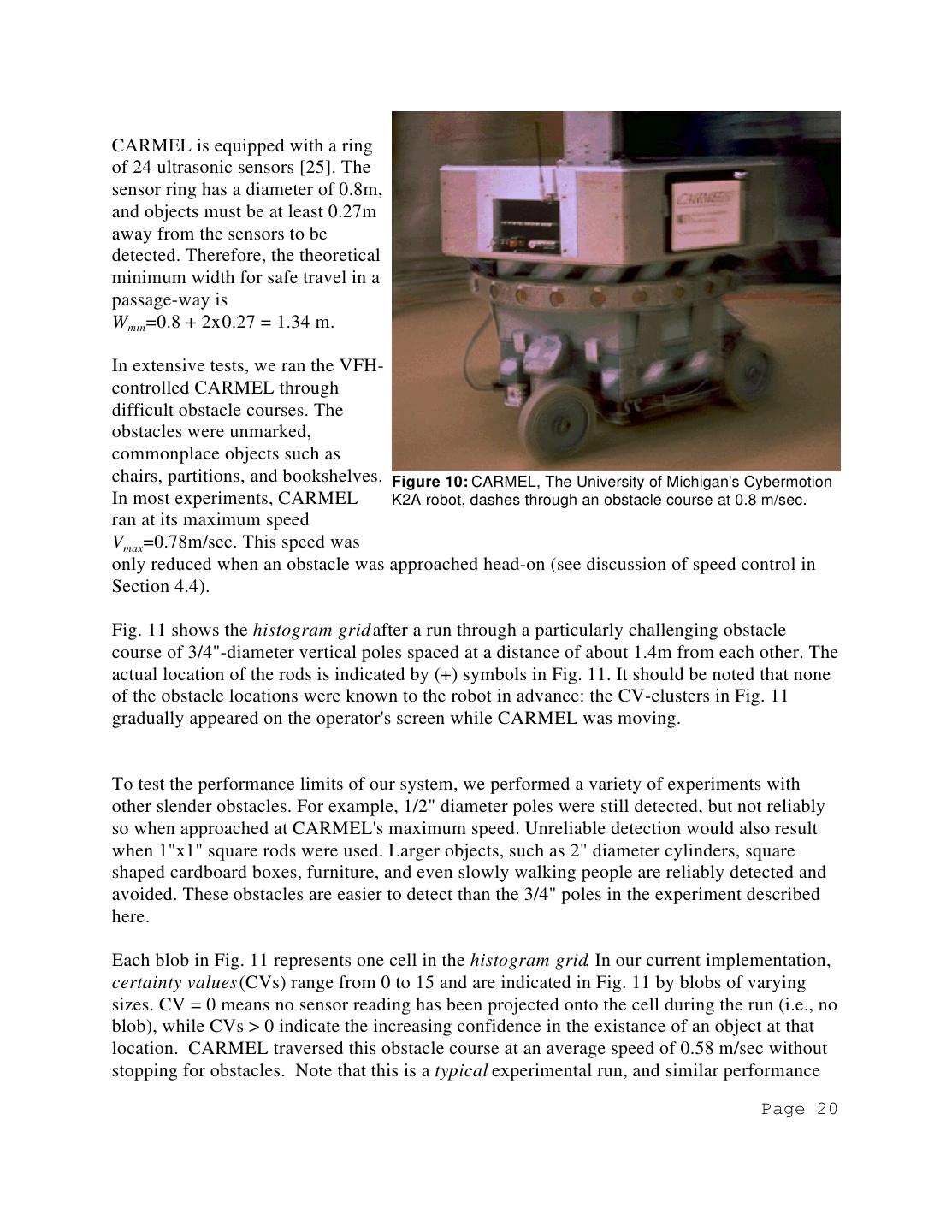
19 .response of the system. Reflexive control (with Brooks as one of its foremost proponents), eliminates cognition altogether. In reflexive control there is no planning and reasoning; nor are there world models. Simple reflexes tie actions to perceptions, resulting in faster response to outside stimuli. At first glance it may seem that our VFH method is a typical example of reactive control, considering the histogram grid world model and even a second model, the polar histogram. However, some distinctions should be made. Our world model, the histogram grid, has two different functional properties, namely a short term effect and a long term effect. The long term effect is provided by the whole histogram grid, as described in Section 3. The information stored in the histogram grid may serve for map building purposes and for the global path planner (see Section 4.5). A large histogram grid, however, is not necessary for our algorithm to work properly. It is the short term effect of the histogram grid that is important for the VFH algorithm. As explained in Section 4.1, only cells within the active window influence the VFH computations. Since the active window travels with the robot, cells are only briefly inside the window and have thus only a temporary (short term)effect. Also, since the ultrasonic sensors are limited to only 2m look-ahead (about the size of the active window), only cells inside the window are updated with sensor information. Therefore, the VFH algorithm would work equally well if all information was lostfrom cells that are outside of the active window. Through the concept of the active window, the histogram grid becomes sort of a "short term memory," where readings are retained briefly (while the active window sweeps through the area) to enhance the accuracy by accumulating multiple sensor readings. In a way, this process is similar to the short term memory associated with human hearing: Without this mechanism, people would hear but not necessarily comprehend all speech. 6. EXPERIMENTAL RESULTS We implemented and tested the VFH method on our mobile robot CARMEL (Computer- Aided Robotics for Maintenance, Emergency, and Life support). CARMEL is based on a commercially available mobile platform [12], as seen in Fig. 10. This platform has a maximum travel speed of Vmax = 0.78 m/sec, a maximum steering rate of Ω = 120 deg/sec, and weighs (in its current configuration) about 125 kg. The platform has a hexagonal structure and a unique three-wheel drive (synchro-drive) that permits omnidirectional steering. A Z-80 on- board computer serves as the low-level controller of the vehicle. Two computers were added: a PC-compatible single-board computer to control the sensors, and a 20 Mhz, 80386-based AT-compatible that runs the VFH algorithm. Page 19 

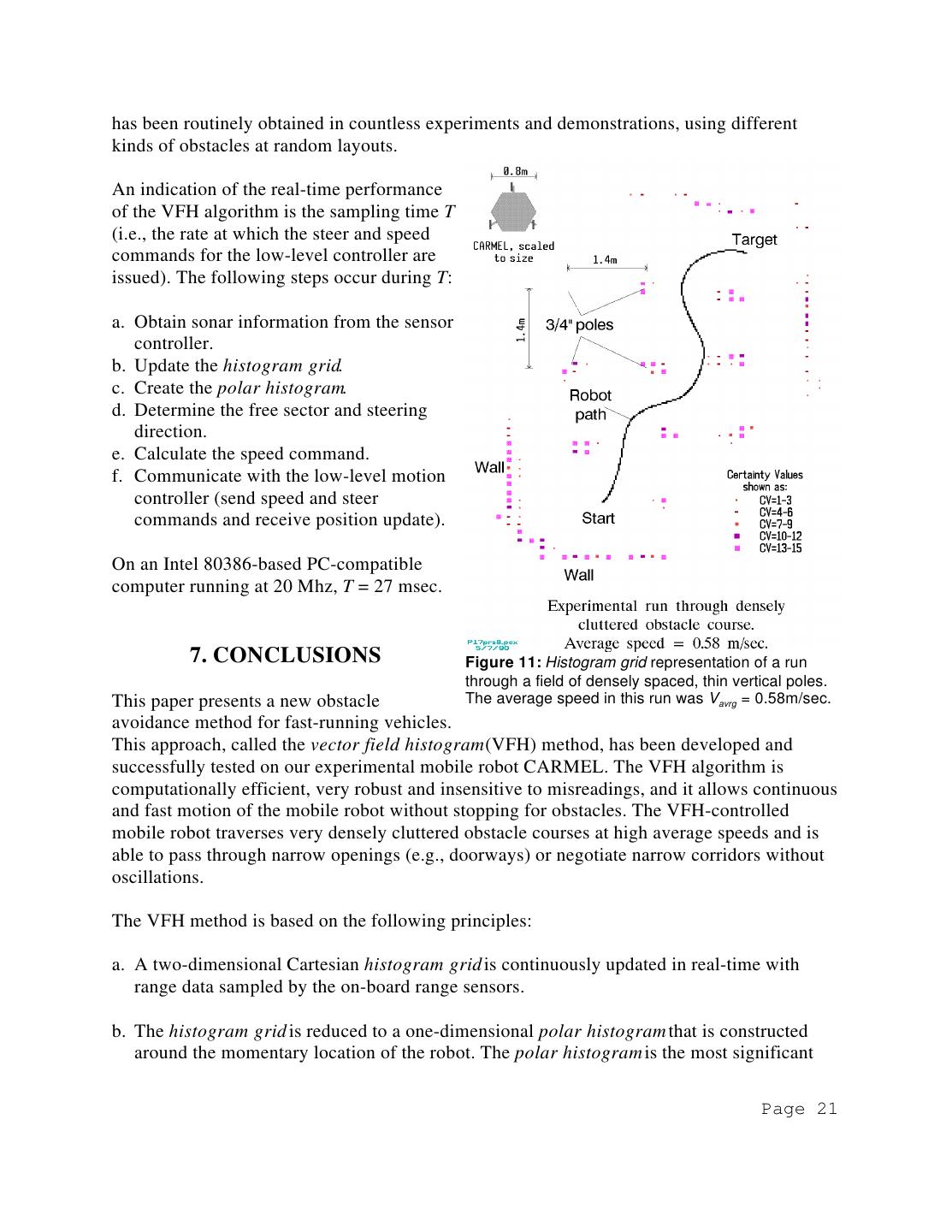
20 .CARMEL is equipped with a ring of 24 ultrasonic sensors [25]. The sensor ring has a diameter of 0.8m, and objects must be at least 0.27m away from the sensors to be detected. Therefore, the theoretical minimum width for safe travel in a passage-way is Wmin=0.8 + 2x0.27 = 1.34 m. In extensive tests, we ran the VFH- controlled CARMEL through difficult obstacle courses. The obstacles were unmarked, commonplace objects such as chairs, partitions, and bookshelves. Figure 10: CARMEL, The University of Michigan's Cybermotion In most experiments, CARMEL K2A robot, dashes through an obstacle course at 0.8 m/sec. ran at its maximum speed Vmax=0.78m/sec. This speed was only reduced when an obstacle was approached head-on (see discussion of speed control in Section 4.4). Fig. 11 shows the histogram grid after a run through a particularly challenging obstacle course of 3/4"-diameter vertical poles spaced at a distance of about 1.4m from each other. The actual location of the rods is indicated by (+) symbols in Fig. 11. It should be noted that none of the obstacle locations were known to the robot in advance: the CV-clusters in Fig. 11 gradually appeared on the operator's screen while CARMEL was moving. To test the performance limits of our system, we performed a variety of experiments with other slender obstacles. For example, 1/2" diameter poles were still detected, but not reliably so when approached at CARMEL's maximum speed. Unreliable detection would also result when 1"x1" square rods were used. Larger objects, such as 2" diameter cylinders, square shaped cardboard boxes, furniture, and even slowly walking people are reliably detected and avoided. These obstacles are easier to detect than the 3/4" poles in the experiment described here. Each blob in Fig. 11 represents one cell in the histogram grid. In our current implementation, certainty values (CVs) range from 0 to 15 and are indicated in Fig. 11 by blobs of varying sizes. CV = 0 means no sensor reading has been projected onto the cell during the run (i.e., no blob), while CVs > 0 indicate the increasing confidence in the existance of an object at that location. CARMEL traversed this obstacle course at an average speed of 0.58 m/sec without stopping for obstacles. Note that this is a typical experimental run, and similar performance Page 20 

21 .has been routinely obtained in countless experiments and demonstrations, using different kinds of obstacles at random layouts. An indication of the real-time performance of the VFH algorithm is the sampling time T (i.e., the rate at which the steer and speed commands for the low-level controller are issued). The following steps occur during T: a. Obtain sonar information from the sensor controller. b. Update the histogram grid. c. Create the polar histogram. d. Determine the free sector and steering direction. e. Calculate the speed command. f. Communicate with the low-level motion controller (send speed and steer commands and receive position update). On an Intel 80386-based PC-compatible computer running at 20 Mhz, T = 27 msec. 7. CONCLUSIONS Figure 11: Histogram grid representation of a run through a field of densely spaced, thin vertical poles. This paper presents a new obstacle The average speed in this run was Vavrg = 0.58m/sec. avoidance method for fast-running vehicles. This approach, called the vector field histogram(VFH) method, has been developed and successfully tested on our experimental mobile robot CARMEL. The VFH algorithm is computationally efficient, very robust and insensitive to misreadings, and it allows continuous and fast motion of the mobile robot without stopping for obstacles. The VFH-controlled mobile robot traverses very densely cluttered obstacle courses at high average speeds and is able to pass through narrow openings (e.g., doorways) or negotiate narrow corridors without oscillations. The VFH method is based on the following principles: a. A two-dimensional Cartesian histogram grid is continuously updated in real-time with range data sampled by the on-board range sensors. b. The histogram grid is reduced to a one-dimensional polar histogram that is constructed around the momentary location of the robot. The polar histogram is the most significant Page 21 

22 . distinction between the VFF and the VFH method as it allows a spatial interpretation (called polar obstacle density) of the robot's instantaneous environment. c. Consecutive sectors with a polar obstacle densitybelow threshold are called "candidate valleys." The candidate valley closest to the target direction is selected for further processing. d. The direction of the center of the selected candidate direction is determined and the steering of the robot is aligned with that direction. e. The speed of the robot is reduced when approaching obstacles head-on. The characteristic behavior of a VFH-controlled mobile robot is best described as follows: The response of the vehicle is dependent on the likelihood for the existence of an obstacle. In the histogram grid, this likelihood is expressed in terms of size and certainty values of a cluster. This information is transformed into height and width of an elevation in the polar histogram. The strength of the VFH method lies thus in its ability to maintain a statistical obstacle representation at both the histogram grid level as well as at the intermediate data level, the polar histogram. This feature makes the VFH method especially suited to the accommodation of inaccurate sensor data, such as that produced by ultrasonic sensors, as well as sensor fusion. Page 22 

23 . 8. REFERENCES 1. Arkin, R. C., "Motor Schema-Based Mobile Robot Navigation." The International Journal of Robotics Research, August 1989, pp. 92-112. 2. Borenstein, J. and Koren, Y., "A Mobile Platform For Nursing Robots." IEEE Trans- actions on Industrial Electronics, Vol. 32, No. 2, 1985, pp. 158-165. 3. Borenstein, J. and Koren, Y., "Motion Control Analysis of a Mobile Robot." Transac- tions of ASME, Journal of Dynamics, Measurement and Control , Vol. 109, No. 2, 1987, pp. 73-79. 4. Borenstein, J. and Koren, Y., "Obstacle Avoidance With Ultrasonic Sensors." IEEE Journal of Robotics and Automation, Vol. RA-4, No. 2, 1988, pp. 213-218. 5. Borenstein, J. and Koren, Y., "Real-time Obstacle Avoidance for Fast Mobile Robots." IEEE Transactions on Systems, Man, and Cybernetics , Vol. 19, No. 5, Sept/Oct 1989, pp. 1179-1187. 6. Borenstein, J. and Koren, Y., "Histogramic In-motion Mapping for Mobile Robot Obstacle Avoidance." IEEE Journal of Robotics and Automation, Vol. 7, No. 4, 1991, pp. 535-539. 7. Borenstein, J. and Koren, Y., "Real-time Map-building for Fast Mobile Robot Obstacle Avoidance." SPIE Symposium on Advances in Intelligent Systems, Mobile Robots ,V Boston, MA, Nov. 4-9, 1990. 8. Brooks, R. A., "A Robust Layered Control System for a Mobile Robot." IEEE Journal of Robotics and Automation, Vol. RA-2, No. 1, 1986, pp. 14-23. 9. Brooks, R. A. and Connell, J. H., "Asynchronous Distributed Control System for a Mobile Robot." Proceedings of the SPIE, Mobile Robots, Vol. 727, 1987, pp. 77-84. 10. Crowley, J. L., "Dynamic World Modeling for an Intelligent Mobile Robot." IEEE Seventh International Conference on Pattern Recognition, Proceedings, Montreal, Canada, July 30-August 2, 1984, pp. 207-210. 11. Crowley, J. L., "World Modeling and Position Estimation for a Mobile Robot Using Ultrasonic Ranging." Proceedings of the 1989 IEEE International Conference on Robotics and Automation. Scottsdale, Arizona, May 14-19, 1989, pp. 674-680. 12. Cybermation, "K2A Mobile Platform." Commercial Offer, 5457 JAE Valley Road, Roanoke, VA 24014, 1987. Page 23 

24 .13. Elfes, A., "Sonar-based Real-World Mapping and Navigation." IEEE Journal of Robotics and Automation, Vol. RA-3, No 3, 1987, pp. 249-265. 14. Flynn, A. M., "Combining Sonar and Infrared Sensors for Mobile Robot Navigation." The International Journal of Robotics Research , Vol. 7, No. 6, December 1988, pp. 5- 14. 15. Newman, W. S. and Hogan, N., "High Speed Robot Control and Obstacle Avoidance Using Dynamic Potential Functions." Proceedings of the 1987 IEEE International Conference on Robotics and Automation,Raleigh, North Carolina, March 31-April 3, 1987, pp. 14-24. 16. Khatib, O., "Real-Time Obstacle Avoidance for Manipulators and Mobile Robots." 1985 IEEE International Conference on Robotics and Automation , St. Louis, Missouri, March 25-28, 1985, pp. 500-505. 17. Koren, Y. and Borenstein, J., "Analysis of Control Methods for Mobile Robot Obstacle Avoidance." Proceedings of the IEEE International Workshop on Intelligent Motion Control, Istanbul, Turkey, August 20-22, 1990, pp. 457-462. 18. Koren, Y. and Borenstein, J., 1991, "Potential Field Methods and Their Inherent Limitations for Mobile Robot Navigation." Proceedings of the IEEE International Conference on Robotics and AutomationSacramento, California, April 7-12, 1991, pp. 1398-1404. 19. Krogh, B. H., "A Generalized Potential Field Approach to Obstacle Avoidance Control." International Robotics Research Conference, Bethlehem, Pennsylvania, August, 1984. 20. Krogh, B. H. and Thorpe, C. E., "Integrated Path Planning and Dynamic Steering Con- trol for Autonomous Vehicles." Proceedings of the 1986 IEEE International Conference on Robotics and Automation, San Francisco, California, April 7-10, 1986, pp. 1664- 1669. 21. Kuc, R. and Barshan, B., "Navigating Vehicles Through an Unstructured Environment With Sonar." Proceedings of the 1989 IEEE International Conference on Robotics and Automation, Scottsdale, Arizona, May 14-19, 1989, pp. 1422-1426. 22. Lumelsky V. and Skewis, T., "A Paradigm for Incorporating Vision in the Robot Navigation Function." Proceedings of the 1988 IEEE Conference on Robotics and Automation, Philadelphia, April 25, 1988, pp. 734-739. 23. Moravec, H. P. and Elfes, A., "High Resolution Maps from Wide Angle Sonar." IEEE Conference on Robotics and Automation, Washington D.C., 1985, pp. 116-121. Page 24 

25 .24. Moravec, H. P., "Sensor Fusion in Certainty Grids for Mobile Robots." AI Magazine, Summer 1988, pp. 61-74. 25. POLAROID Corporation, Ultrasonic Components Group, 119 Windsor Street, Cambridge, Massachusetts 02139, 1990. 26. Raschke, U. and Borenstein, J., "A Comparisson of Grid-type Map-building Techniques by Index of Performance." Proceedings of the 1990 IEEE International Conference on Robotics and Automation, Cincinnati, Ohio, May 13-18, 1990. 27. Thorpe, C. F., "Path Relaxation: Path Planning for a Mobile Robot." Carnegie-Mellon University, The Robotics Institute, Mobile Robots Laboratory, Autonomous Mobile Robots, Annual Report 1985, pp. 39-42. 28. Weisbin, C. R., de Saussure, G., and Kammer, D., "SELF-CONTROLLED. A Real- Time Expert System for an Autonomous Mobile Robot." Computers in Mechanical Engineering, September, 1986, pp. 12-19. 29. Zhao, Y., BeMent, S. L., and Borenstein, J., "Dynamic Path Planning for Mobile Robot Real-time Navigation." Twelfth IASTED International Symposium on Robotics and Manufacturing, Santa Barbara, California, November 13-15, 1989. Footnotes 1. We use the term "probability" in the literal sense of "likelihood." 2. For symmetrically shaped vehicles, the VCP is easily defined as the geometric center of the vehicle. For rectangular vehicles, it is possible to chose two VCPs, e.g., one each at the center-point of the front and rear axles. Page 25