Deeply-Recursive Convolutional Network for Image Super-Resolution

1 . Deeply-Recursive Convolutional Network for Image Super-Resolution Jiwon Kim, Jung Kwon Lee and Kyoung Mu Lee Department of ECE, ASRI, Seoul National University, Korea {j.kim, deruci, kyoungmu}@snu.ac.kr arXiv:1511.04491v2 [cs.CV] 11 Nov 2016 Abstract required. Second, the model becomes too huge to be stored and retrieved. We propose an image super-resolution method (SR) us- ing a deeply-recursive convolutional network (DRCN). Our To resolve these issues, we use a deeply-recursive con- network has a very deep recursive layer (up to 16 recur- volutional network (DRCN). DRCN repeatedly applies the sions). Increasing recursion depth can improve perfor- same convolutional layer as many times as desired. The mance without introducing new parameters for additional number of parameters do not increase while more recur- convolutions. Albeit advantages, learning a DRCN is very sions are performed. Our network has the receptive field hard with a standard gradient descent method due to ex- of 41 by 41 and this is relatively large compared to SRCNN ploding/vanishing gradients. To ease the difficulty of train- [5] (13 by 13). While DRCN has good properties, we find ing, we propose two extensions: recursive-supervision and that DRCN optimized with the widely-used stochastic gra- skip-connection. Our method outperforms previous meth- dient descent method does not easily converge. This is due ods by a large margin. to exploding/vanishing gradients [1]. Learning long-range dependencies between pixels with a single weight layer is very difficult. 1. Introduction For image super-resolution (SR), receptive field of a con- We propose two approaches to ease the difficulty of volutional network determines the amount of contextual training (Figure 3(a)). First, all recursions are supervised. information that can be exploited to infer missing high- Feature maps after each recursion are used to reconstruct the frequency components. For example, if there exists a pat- target high-resolution image (HR). Reconstruction method tern with smoothed edges contained in a receptive field, it is (layers dedicated to reconstruction) is the same for all recur- plausible that the pattern is recognized and edges are appro- sions. As each recursion leads to a different HR prediction, priately sharpened. As SR is an ill-posed inverse problem, we combine all predictions resulting from different levels of collecting and analyzing more neighbor pixels can possibly recursions to deliver a more accurate final prediction. The give more clues on what may be lost by downsampling. second proposal is to use a skip-connection from input to Deep convolutional networks (DCN) succeeding in var- the reconstruction layer. In SR, a low-resolution image (in- ious computer vision tasks often use very large recep- put) and a high-resolution image (output) share the same tive fields (224x224 common in ImageNet classification information to a large extent. Exact copy of input, how- [13, 24]). Among many approaches to widen the receptive ever, is likely to be attenuated during many forward passes. field, increasing network depth is one possible way: a con- We explicitly connect the input to the layers for output re- volutional (conv.) layer with filter size larger than a 1 × 1 or construction. This is particularly effective when input and a pooling (pool.) layer that reduces the dimension of inter- output are highly correlated. mediate representation can be used. Both approaches have drawbacks: a conv. layer introduces more parameters and a pool. layer typically discards some pixel-wise information. Contributions In summary, we propose an image super- For image restoration problems such as super-resolution resolution method deeply recursive in nature. It utilizes a and denoising, image details are very important. Therefore, very large context compared to previous SR methods with most deep-learning approaches for such problems do not only a single recursive layer. We improve the simple recur- use pooling. Increasing depth by adding a new weight layer sive network in two ways: recursive-supervision and skip- basically introduces more parameters. Two problems can connection. Our method demonstrates state-of-the-art per- arise. First, overfitting is highly likely. More data are now formance in common benchmarks. 1 

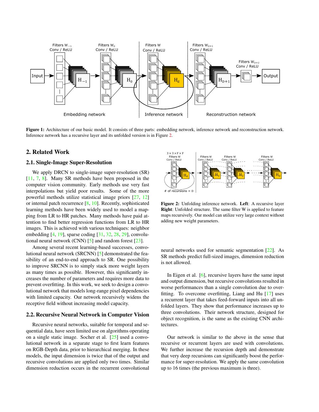
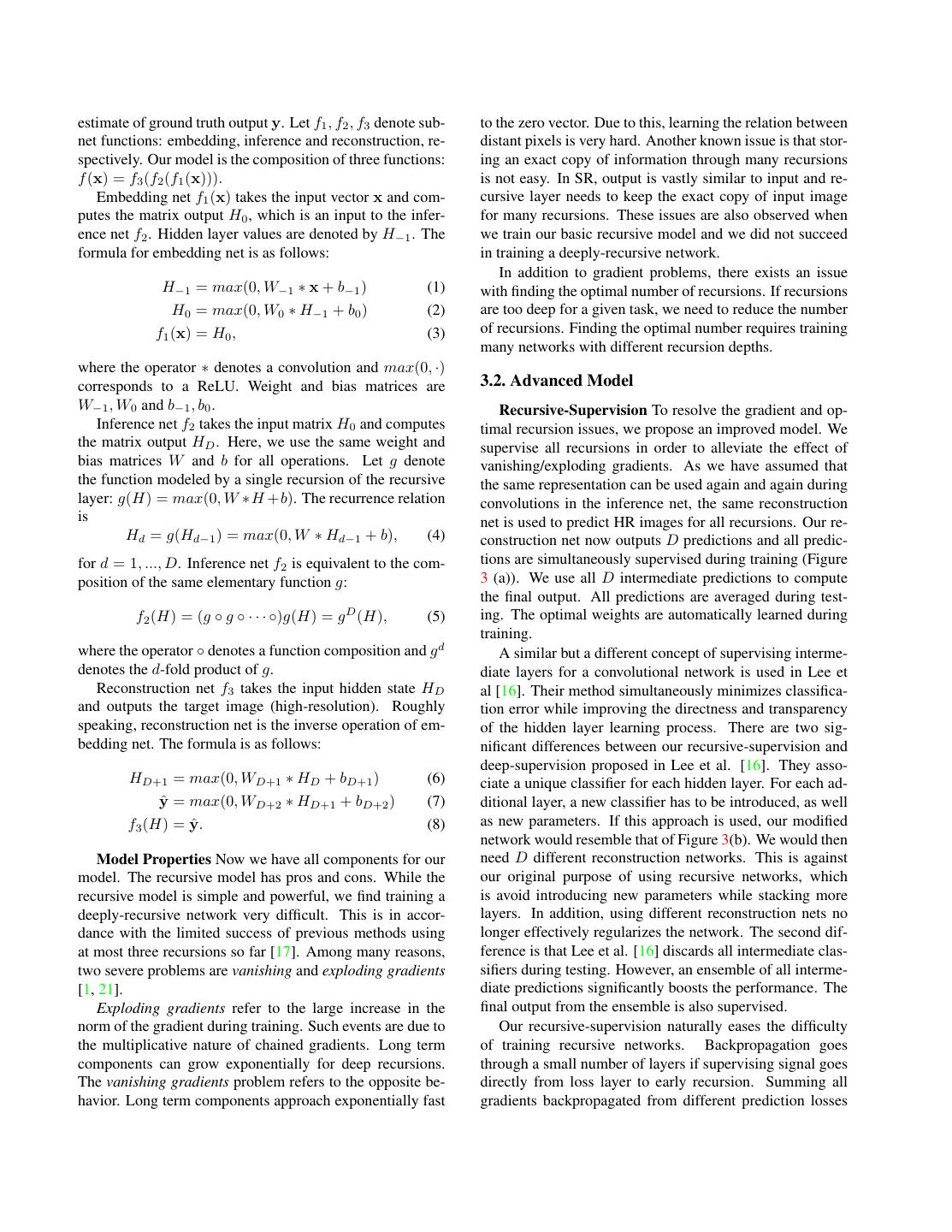
2 . Filters W－1 Filters W0 Filters W Filters WD＋1 Conv / ReLU Conv / ReLU Conv / ReLU Conv / ReLU Filters WD＋2 Conv / ReLU Input Output H－1 H0 Hd HD＋1 Embedding network Inference network Reconstruction network Figure 1: Architecture of our basic model. It consists of three parts: embedding network, inference network and reconstruction network. Inference network has a recursive layer and its unfolded version is in Figure 2. 2. Related Work 3 × 3 × F × F Filters W Filters W Filters W Filters W Conv / ReLU Conv / ReLU Conv / ReLU Conv / ReLU 2.1. Single-Image Super-Resolution We apply DRCN to single-image super-resolution (SR) Hd H1 H2 HD [11, 7, 8]. Many SR methods have been proposed in the computer vision community. Early methods use very fast interpolations but yield poor results. Some of the more # of recursions = D powerful methods utilize statistical image priors [27, 12] or internal patch recurrence [8, 10]. Recently, sophisticated Figure 2: Unfolding inference network. Left: A recursive layer learning methods have been widely used to model a map- Right: Unfolded structure. The same filter W is applied to feature ping from LR to HR patches. Many methods have paid at- maps recursively. Our model can utilize very large context without tention to find better regression functions from LR to HR adding new weight parameters. images. This is achieved with various techniques: neighbor embedding [4, 19], sparse coding [31, 32, 28, 29], convolu- tional neural network (CNN) [5] and random forest [23]. Among several recent learning-based successes, convo- neural networks used for semantic segmentation [22]. As lutional neural network (SRCNN) [5] demonstrated the fea- SR methods predict full-sized images, dimension reduction sibility of an end-to-end approach to SR. One possibility is not allowed. to improve SRCNN is to simply stack more weight layers as many times as possible. However, this significantly in- In Eigen et al. [6], recursive layers have the same input creases the number of parameters and requires more data to and output dimension, but recursive convolutions resulted in prevent overfitting. In this work, we seek to design a convo- worse performances than a single convolution due to over- lutional network that models long-range pixel dependencies fitting. To overcome overfitting, Liang and Hu [17] uses with limited capacity. Our network recursively widens the a recurrent layer that takes feed-forward inputs into all un- receptive field without increasing model capacity. folded layers. They show that performance increases up to three convolutions. Their network structure, designed for 2.2. Recursive Neural Network in Computer Vision object recognition, is the same as the existing CNN archi- Recursive neural networks, suitable for temporal and se- tectures. quential data, have seen limited use on algorithms operating on a single static image. Socher et al. [25] used a convo- Our network is similar to the above in the sense that lutional network in a separate stage to first learn features recursive or recurrent layers are used with convolutions. on RGB-Depth data, prior to hierarchical merging. In these We further increase the recursion depth and demonstrate models, the input dimension is twice that of the output and that very deep recursions can significantly boost the perfor- recursive convolutions are applied only two times. Similar mance for super-resolution. We apply the same convolution dimension reduction occurs in the recurrent convolutional up to 16 times (the previous maximum is three). 

3 . (a) Skip connection Output Output1d w1 wd－1 Output d－1 Recon wd Final Output d Output Net Output d＋1 wd＋1 Embed Input H1 Hd－1 Hd Hd＋1 HD Output D wD Net : Shared filters W (b) Final Local outputs Outputd-1 Output 1 Output Output d－1 d-1 Output Output dd Output Output d＋1 d+1 Outputd+1 Output D Output Recon Net 1 Recon Net d－1 Recon Net d Recon Net d＋1 Recon Net D Embed Input H1 Hd－1 Hd Hd＋1 HD Net (c) Embed Recon H11 Output Output1d Net 1 Net 1 Embed Recon Net d－1 Hd－1 1 Hd－1 d－1 Net d－1 Output d－1 Embed Recon Final Input Hd1 Hdd－1 Hdd Output d Net d Net d Output Embed Recon H1d＋1 d＋1 Hd－1 Hdd＋1 d＋1 Hd＋1 Output d＋1 Net d＋1 Net d＋1 Embed Recon Net D H1D D Hd－1 HdD D Hd＋1 HDD Net D Output D Figure 3: (a): Our final (advanced) model with recursive-supervision and skip-connection. The reconstruction network is shared for recursive predictions. We use all predictions from the intermediate recursion to obtain the final output. (b): Applying deep-supervision [16] to our basic model. Unlike in (a), the model in (b) uses different reconstruction networks for recursions and more parameters are used. (c): An example of expanded structure of (a) without parameter sharing (no recursion). The number of weight parameters is proportional to the depth squared. 3. Proposed Method 1 × 1, the receptive field is widened with every recursion. While feature maps from the final application of the recur- 3.1. Basic Model sive layer represent the high-resolution image, transforming them (multi-channel) back into the original image space (1 Our first model, outlined in Figure 1, consists of three or 3-channel) is necessary. This is done by the reconstruc- sub-networks: embedding, inference and reconstruction tion net. networks. The embedding net is used to represent the given image as feature maps ready for inference. Next, the infer- We have a single hidden layer for each sub-net. Only the ence net solves the task. Once inference is done, final fea- layer for the inference net is recursive. Other sub-nets are ture maps in the inference net are fed into the reconstruction vastly similar to the standard mutilayer perceptrons (MLP) net to generate the output image. with a single hidden layer. For MLP, full connection of F The embedding net takes the input image (grayscale or neurons is equivalent to a convolution with 1 × 1 × F × F . RGB) and represents it as a set of feature maps. Intermedi- In our sub-nets, we use 3×3×F ×F filters. For embedding ate representation used to pass information to the inference net, we use 3×3 filters because image gradients are more in- net largely depends on how the inference net internally rep- formative than the raw intensities for super-resolution. For resent its feature maps in its hidden layers. Learning this inference net, 3 × 3 convolutions imply that hidden states representation is done end-to-end altogether with learning are passed to adjacent pixels only. Reconstruction net also other sub-networks. Inference net is the main component takes direct neighbors into account. that solves the task of super-resolution. Analyzing a large Mathematical Formulation The network takes an in- image region is done by a single recursive layer. Each re- terpolated input image (to the desired size) as input x and cursion applies the same convolution followed by a rectified predicts the target image y as in SRCNN [5]. Our goal is to linear unit (Figure 2). With convolution filters larger than learn a model f that predicts values y ˆ = f (x), where y ˆ is its 

4 .estimate of ground truth output y. Let f1 , f2 , f3 denote sub- to the zero vector. Due to this, learning the relation between net functions: embedding, inference and reconstruction, re- distant pixels is very hard. Another known issue is that stor- spectively. Our model is the composition of three functions: ing an exact copy of information through many recursions f (x) = f3 (f2 (f1 (x))). is not easy. In SR, output is vastly similar to input and re- Embedding net f1 (x) takes the input vector x and com- cursive layer needs to keep the exact copy of input image putes the matrix output H0 , which is an input to the infer- for many recursions. These issues are also observed when ence net f2 . Hidden layer values are denoted by H−1 . The we train our basic recursive model and we did not succeed formula for embedding net is as follows: in training a deeply-recursive network. In addition to gradient problems, there exists an issue H−1 = max(0, W−1 ∗ x + b−1 ) (1) with finding the optimal number of recursions. If recursions H0 = max(0, W0 ∗ H−1 + b0 ) (2) are too deep for a given task, we need to reduce the number f1 (x) = H0 , (3) of recursions. Finding the optimal number requires training many networks with different recursion depths. where the operator ∗ denotes a convolution and max(0, ·) corresponds to a ReLU. Weight and bias matrices are 3.2. Advanced Model W−1 , W0 and b−1 , b0 . Recursive-Supervision To resolve the gradient and op- Inference net f2 takes the input matrix H0 and computes timal recursion issues, we propose an improved model. We the matrix output HD . Here, we use the same weight and supervise all recursions in order to alleviate the effect of bias matrices W and b for all operations. Let g denote vanishing/exploding gradients. As we have assumed that the function modeled by a single recursion of the recursive the same representation can be used again and again during layer: g(H) = max(0, W ∗H +b). The recurrence relation convolutions in the inference net, the same reconstruction is net is used to predict HR images for all recursions. Our re- Hd = g(Hd−1 ) = max(0, W ∗ Hd−1 + b), (4) construction net now outputs D predictions and all predic- for d = 1, ..., D. Inference net f2 is equivalent to the com- tions are simultaneously supervised during training (Figure position of the same elementary function g: 3 (a)). We use all D intermediate predictions to compute the final output. All predictions are averaged during test- f2 (H) = (g ◦ g ◦ · · · ◦)g(H) = g D (H), (5) ing. The optimal weights are automatically learned during training. where the operator ◦ denotes a function composition and g d A similar but a different concept of supervising interme- denotes the d-fold product of g. diate layers for a convolutional network is used in Lee et Reconstruction net f3 takes the input hidden state HD al [16]. Their method simultaneously minimizes classifica- and outputs the target image (high-resolution). Roughly tion error while improving the directness and transparency speaking, reconstruction net is the inverse operation of em- of the hidden layer learning process. There are two sig- bedding net. The formula is as follows: nificant differences between our recursive-supervision and deep-supervision proposed in Lee et al. [16]. They asso- HD+1 = max(0, WD+1 ∗ HD + bD+1 ) (6) ciate a unique classifier for each hidden layer. For each ad- ˆ = max(0, WD+2 ∗ HD+1 + bD+2 ) y (7) ditional layer, a new classifier has to be introduced, as well ˆ. f3 (H) = y (8) as new parameters. If this approach is used, our modified network would resemble that of Figure 3(b). We would then Model Properties Now we have all components for our need D different reconstruction networks. This is against model. The recursive model has pros and cons. While the our original purpose of using recursive networks, which recursive model is simple and powerful, we find training a is avoid introducing new parameters while stacking more deeply-recursive network very difficult. This is in accor- layers. In addition, using different reconstruction nets no dance with the limited success of previous methods using longer effectively regularizes the network. The second dif- at most three recursions so far [17]. Among many reasons, ference is that Lee et al. [16] discards all intermediate clas- two severe problems are vanishing and exploding gradients sifiers during testing. However, an ensemble of all interme- [1, 21]. diate predictions significantly boosts the performance. The Exploding gradients refer to the large increase in the final output from the ensemble is also supervised. norm of the gradient during training. Such events are due to Our recursive-supervision naturally eases the difficulty the multiplicative nature of chained gradients. Long term of training recursive networks. Backpropagation goes components can grow exponentially for deep recursions. through a small number of layers if supervising signal goes The vanishing gradients problem refers to the opposite be- directly from loss layer to early recursion. Summing all havior. Long term components approach exponentially fast gradients backpropagated from different prediction losses 

5 .gives a smoothing effect. The adversarial effect of vanish- mediate predictions: ing/exploding gradients along one backpropagation path is D alleviated. ˆ= y wd · y ˆd. (10) Moreover, the importance of picking the optimal number d=1 of recursions is reduced as our supervision enables utilizing predictions from all intermediate layers. If recursions are where wd denotes the weights of predictions reconstructed too deep for the given task, we expect the weight for late from each intermediate hidden state during recursion. predictions to be low while early predictions receive high These weights are learned during training. weights. 3.3. Training By looking at weights of predictions, we can figure out the marginal gain from additional recursions. Objective We now describe the training objective used We present an expanded CNN structure of our model for to find optimal parameters of our model. Given a training illustration purposes in Figure 3(c). If parameters are not dataset {x(i) , y(i) }N i=1 , our goal is to find the best model f allowed to be shared and CNN chains vary their depths, the that accurately predicts values y ˆ = f (x). number of free parameters grows fast (quadratically). In the least-squares regression setting, typical in SR, the mean squared error 21 ||y − f (x)||2 averaged over the train- Skip-Connection Now we describe our second exten- ing set is minimized. This favors high Peak Signal-to-Noise sion: skip-connection. For SR, input and output images are Ratio (PSNR), a widely-used evaluation criteria. highly correlated. Carrying most if not all of input values With recursive-supervision, we have D + 1 objectives until the end of the network is inevitable but very inefficient. to minimize: supervising D outputs from recursions and Due to gradient problems, exactly learning a simple linear the final output. For intermediate outputs, we have the loss relation between input and output is very difficult if many function recursions exist in between them. D N We add a layer skip [3] from input to the reconstruction 1 (i) net. Adding layer skips is successfully used for a semantic l1 (θ) = ||y(i) − y ˆ d ||2 , (11) 2DN d=1 i=1 segmentation network [18] and we employ a similar idea. Now input image is directly fed into the reconstruction net (i) where θ denotes the parameter set and y ˆ d is the output whenever it is used during recursions. Our skip-connection from the d-th recursion. For the final output, we have has two advantages. First, network capacity to store the input signal during recursions is saved. Second, the exact N D 1 (i) copy of input signal can be used during target prediction. l2 (θ) = ||y(i) − ˆ d ||2 wd · y (12) 2N Our skip-connection is simple yet very effective. In i=1 d=1 super-resolution, LR and HR images are vastly similar. In Now we give the final loss function L(θ). The training is most regions, differences are zero and only small number regularized by weight decay (L2 penalty multiplied by β). of locations have non-zero values. For this reason, sev- eral super-resolution methods [28, 29, 19, 2] predict image L(θ) = αl1 (θ) + (1 − α)l2 (θ) + β||θ||2 , (13) details only. Similarly, we find that this domain-specific knowledge significantly improves our learning procedure. where α denotes the importance of the companion objective Mathematical Formulation Each intermediate predic- on the intermediate outputs and β denotes the multiplier of tion under recursive-supervision (Figure 3(a)) is weight decay. Setting α high makes the training procedure stable as early recursions easily converge. As training pro- ˆ d = f3 (x, g (d) (f1 (x))), y (9) gresses, α decays to boost the performance of the final out- put. Training is carried out by optimizing the regression ob- for d = 1, 2, . . . , D, where f3 now takes two inputs, jective using mini-batch gradient descent based on back- one from skip-connection. Reconstruction net with skip- propagation (LeCun et al. [15]). We implement our model connection can take various functional forms. For exam- using the MatConvNet1 package [30]. ple, input can be concatenated to the feature maps Hd . As the input is an interpolated input image (roughly speaking, 4. Experimental Results ˆ ≈ x), we find f3 (x, Hd ) = x + f3 (Hd ) is enough for y our purpose. More sophisticated functions for merging two In this section, we evaluate the performance of our inputs to f3 will be explored in the future. method on several datasets. We first describe datasets used Now, the final output is the weighted average of all inter- 1 http://www.vlfeat.org/matconvnet/ 

6 . Ground Truth A+ [29] SRCNN [5] RFL [23] SelfEx [10] DRCN (Ours) (PSNR, SSIM) (29.83, 0.9102) (29.97, 0.9092) (29.61, 0.9026) (30.73, 0.9193) (32.17, 0.9350) Figure 4: Super-resolution results of “img082”(Urban100) with scale factor ×4. Line is straightened and sharpened in our result, whereas other methods give blurry lines. Our result seems visually pleasing. Ground Truth A+ [29] SRCNN [5] RFL [23] SelfEx [10] DRCN (Ours) (PSNR, SSIM) (23.53, 0.6977) (23.79, 0.7087) (23.53, 0.6943) (23.52, 0.7006) (24.36, 0.7399) Figure 5: Super-resolution results of “134035” (B100) with scale factor ×4. Our result shows a clear separation between branches while in other methods, branches are not well separated. Ground Truth A+ [29] SRCNN [5] RFL [23] SelfEx [10] DRCN (Ours) (PSNR, SSIM) (26.09, 0.9342) (27.01, 0.9365) (25.91, 0.9254) (27.10, 0.9483) (27.66, 0.9608) Figure 6: Super-resolution results of “ppt3” (Set14) with scale factor ×3. Texts in DRCN are sharp while, in other methods, character edges are blurry. 

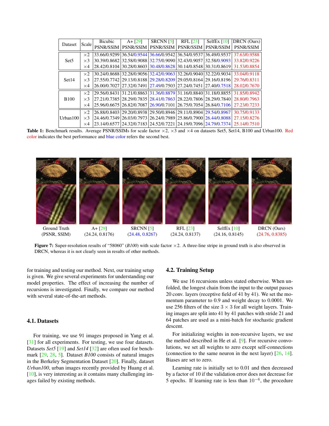
7 . Bicubic A+ [29] SRCNN [5] RFL [23] SelfEx [10] DRCN (Ours) Dataset Scale PSNR/SSIM PSNR/SSIM PSNR/SSIM PSNR/SSIM PSNR/SSIM PSNR/SSIM ×2 33.66/0.9299 36.54/0.9544 36.66/0.9542 36.54/0.9537 36.49/0.9537 37.63/0.9588 Set5 ×3 30.39/0.8682 32.58/0.9088 32.75/0.9090 32.43/0.9057 32.58/0.9093 33.82/0.9226 ×4 28.42/0.8104 30.28/0.8603 30.48/0.8628 30.14/0.8548 30.31/0.8619 31.53/0.8854 ×2 30.24/0.8688 32.28/0.9056 32.42/0.9063 32.26/0.9040 32.22/0.9034 33.04/0.9118 Set14 ×3 27.55/0.7742 29.13/0.8188 29.28/0.8209 29.05/0.8164 29.16/0.8196 29.76/0.8311 ×4 26.00/0.7027 27.32/0.7491 27.49/0.7503 27.24/0.7451 27.40/0.7518 28.02/0.7670 ×2 29.56/0.8431 31.21/0.8863 31.36/0.8879 31.16/0.8840 31.18/0.8855 31.85/0.8942 B100 ×3 27.21/0.7385 28.29/0.7835 28.41/0.7863 28.22/0.7806 28.29/0.7840 28.80/0.7963 ×4 25.96/0.6675 26.82/0.7087 26.90/0.7101 26.75/0.7054 26.84/0.7106 27.23/0.7233 ×2 26.88/0.8403 29.20/0.8938 29.50/0.8946 29.11/0.8904 29.54/0.8967 30.75/0.9133 Urban100 ×3 24.46/0.7349 26.03/0.7973 26.24/0.7989 25.86/0.7900 26.44/0.8088 27.15/0.8276 ×4 23.14/0.6577 24.32/0.7183 24.52/0.7221 24.19/0.7096 24.79/0.7374 25.14/0.7510 Table 1: Benchmark results. Average PSNR/SSIMs for scale factor ×2, ×3 and ×4 on datasets Set5, Set14, B100 and Urban100. Red color indicates the best performance and blue color refers the second best. Ground Truth A+ [29] SRCNN [5] RFL [23] SelfEx [10] DRCN (Ours) (PSNR, SSIM) (24.24, 0.8176) (24.48, 0.8267) (24.24, 0.8137) (24.16, 0.8145) (24.76, 0.8385) Figure 7: Super-resolution results of “58060” (B100) with scale factor ×2. A three-line stripe in ground truth is also observed in DRCN, whereas it is not clearly seen in results of other methods. for training and testing our method. Next, our training setup 4.2. Training Setup is given. We give several experiments for understanding our model properties. The effect of increasing the number of We use 16 recursions unless stated otherwise. When un- recursions is investigated. Finally, we compare our method folded, the longest chain from the input to the output passes with several state-of-the-art methods. 20 conv. layers (receptive field of 41 by 41). We set the mo- mentum parameter to 0.9 and weight decay to 0.0001. We use 256 filters of the size 3 × 3 for all weight layers. Train- ing images are split into 41 by 41 patches with stride 21 and 4.1. Datasets 64 patches are used as a mini-batch for stochastic gradient descent. For training, we use 91 images proposed in Yang et al. For initializing weights in non-recursive layers, we use [31] for all experiments. For testing, we use four datasets. the method described in He et al. [9]. For recursive convo- Datasets Set5 [19] and Set14 [32] are often used for bench- lutions, we set all weights to zero except self-connections mark [29, 28, 5]. Dataset B100 consists of natural images (connection to the same neuron in the next layer) [26, 14]. in the Berkeley Segmentation Dataset [20]. Finally, dataset Biases are set to zero. Urban100, urban images recently provided by Huang et al. Learning rate is initially set to 0.01 and then decreased [10], is very interesting as it contains many challenging im- by a factor of 10 if the validation error does not decrease for ages failed by existing methods. 5 epochs. If learning rate is less than 10−6 , the procedure 

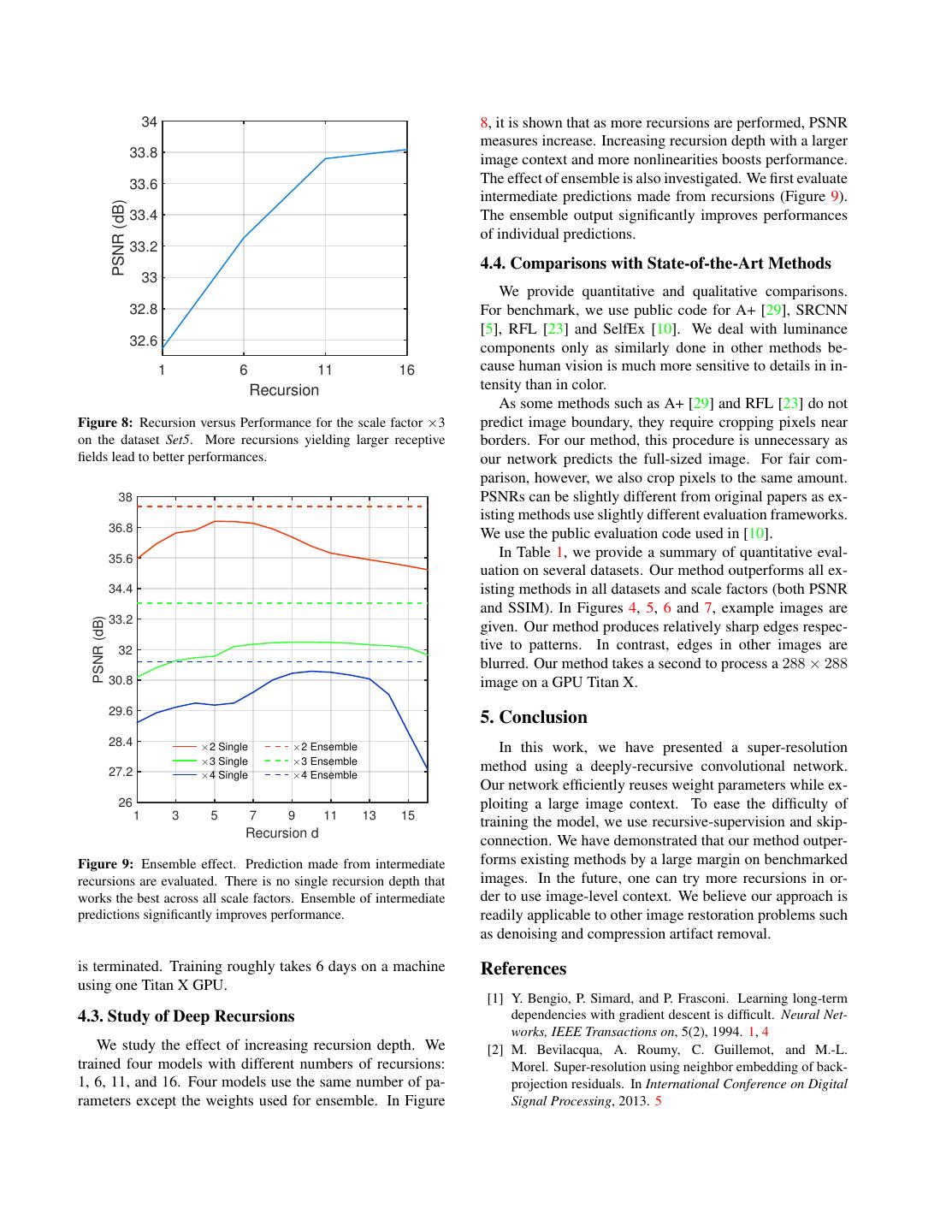
8 . 34 8, it is shown that as more recursions are performed, PSNR measures increase. Increasing recursion depth with a larger 33.8 image context and more nonlinearities boosts performance. 33.6 The effect of ensemble is also investigated. We first evaluate intermediate predictions made from recursions (Figure 9). PSNR (dB) 33.4 The ensemble output significantly improves performances of individual predictions. 33.2 4.4. Comparisons with State-of-the-Art Methods 33 We provide quantitative and qualitative comparisons. 32.8 For benchmark, we use public code for A+ [29], SRCNN [5], RFL [23] and SelfEx [10]. We deal with luminance 32.6 components only as similarly done in other methods be- 1 6 11 16 cause human vision is much more sensitive to details in in- Recursion tensity than in color. As some methods such as A+ [29] and RFL [23] do not Figure 8: Recursion versus Performance for the scale factor ×3 predict image boundary, they require cropping pixels near on the dataset Set5. More recursions yielding larger receptive borders. For our method, this procedure is unnecessary as fields lead to better performances. our network predicts the full-sized image. For fair com- parison, however, we also crop pixels to the same amount. 38 PSNRs can be slightly different from original papers as ex- isting methods use slightly different evaluation frameworks. 36.8 We use the public evaluation code used in [10]. 35.6 In Table 1, we provide a summary of quantitative eval- uation on several datasets. Our method outperforms all ex- 34.4 isting methods in all datasets and scale factors (both PSNR and SSIM). In Figures 4, 5, 6 and 7, example images are 33.2 PSNR (dB) given. Our method produces relatively sharp edges respec- 32 tive to patterns. In contrast, edges in other images are blurred. Our method takes a second to process a 288 × 288 30.8 image on a GPU Titan X. 29.6 5. Conclusion 28.4 #2 Single #2 Ensemble In this work, we have presented a super-resolution #3 Single #3 Ensemble 27.2 method using a deeply-recursive convolutional network. #4 Single #4 Ensemble Our network efficiently reuses weight parameters while ex- 26 ploiting a large image context. To ease the difficulty of 1 3 5 7 9 11 13 15 training the model, we use recursive-supervision and skip- Recursion d connection. We have demonstrated that our method outper- Figure 9: Ensemble effect. Prediction made from intermediate forms existing methods by a large margin on benchmarked recursions are evaluated. There is no single recursion depth that images. In the future, one can try more recursions in or- works the best across all scale factors. Ensemble of intermediate der to use image-level context. We believe our approach is predictions significantly improves performance. readily applicable to other image restoration problems such as denoising and compression artifact removal. is terminated. Training roughly takes 6 days on a machine References using one Titan X GPU. [1] Y. Bengio, P. Simard, and P. Frasconi. Learning long-term 4.3. Study of Deep Recursions dependencies with gradient descent is difficult. Neural Net- works, IEEE Transactions on, 5(2), 1994. 1, 4 We study the effect of increasing recursion depth. We [2] M. Bevilacqua, A. Roumy, C. Guillemot, and M.-L. trained four models with different numbers of recursions: Morel. Super-resolution using neighbor embedding of back- 1, 6, 11, and 16. Four models use the same number of pa- projection residuals. In International Conference on Digital rameters except the weights used for ensemble. In Figure Signal Processing, 2013. 5 

9 . [3] C. M. Bishop. Pattern recognition and machine learning. [23] S. Schulter, C. Leistner, and H. Bischof. Fast and accu- springer, 2006. 5 rate image upscaling with super-resolution forests. In CVPR, [4] H. Chang, D.-Y. Yeung, and Y. Xiong. Super-resolution 2015. 2, 6, 7, 8 through neighbor embedding. In CVPR, 2004. 2 [24] K. Simonyan and A. Zisserman. Very deep convolutional [5] C. Dong, C. C. Loy, K. He, and X. Tang. Image super- networks for large-scale image recognition. In ICLR, 2015. resolution using deep convolutional networks. TPAMI, 2014. 1 1, 2, 3, 6, 7, 8 [25] R. Socher, B. Huval, B. Bath, C. D. Manning, and A. Y. Ng. [6] D. Eigen, J. Rolfe, R. Fergus, and Y. LeCun. Understanding Convolutional-recursive deep learning for 3d object classifi- deep architectures using a recursive convolutional network. cation. In NIPS, 2012. 2 In ICLR Workshop, 2014. 2 [26] R. Socher, B. Huval, C. D. Manning, and A. Y. Ng. Semantic [7] W. T. Freeman, E. C. Pasztor, and O. T. Carmichael. Learn- compositionality through recursive matrix-vector spaces. In ing low-level vision. IJCV, 2000. 2 EMNLP-CoNLL, 2012. 7 [8] D. Glasner, S. Bagon, and M. Irani. Super-resolution from a [27] J. Sun, Z. Xu, and H.-Y. Shum. Image super-resolution using single image. In ICCV, 2009. 2 gradient profile prior. In CVPR, 2008. 2 [9] K. He, X. Zhang, S. Ren, and J. Sun. Delving deep into [28] R. Timofte, V. De, and L. V. Gool. Anchored neighborhood rectifiers: Surpassing human-level performance on imagenet regression for fast example-based super-resolution. In ICCV, classification. In ICCV, 2015. 7 2013. 2, 5, 7 [10] J.-B. Huang, A. Singh, and N. Ahuja. Single image super- [29] R. Timofte, V. De Smet, and L. Van Gool. A+: Adjusted resolution using transformed self-exemplars. In CVPR, 2015. anchored neighborhood regression for fast super-resolution. 2, 6, 7, 8 In ACCV, 2014. 2, 5, 6, 7, 8 [11] M. Irani and S. Peleg. Improving resolution by image reg- [30] A. Vedaldi and K. Lenc. Matconvnet – convolutional neural istration. CVGIP: Graphical models and image processing, networks for matlab. CoRR, abs/1412.4564, 2014. 5 53(3), 1991. 2 [31] J. Yang, J. Wright, T. S. Huang, and Y. Ma. Image super- resolution via sparse representation. TIP, 2010. 2, 7 [12] K. I. Kim and Y. Kwon. Single-image super-resolution using sparse regression and natural image prior. TPAMI, 2010. 2 [32] R. Zeyde, M. Elad, and M. Protter. On single image scale- up using sparse-representations. In Curves and Surfaces. [13] A. Krizhevsky, I. Sutskever, and G. E. Hinton. Imagenet Springer, 2012. 2, 7 classification with deep convolutional neural networks. In NIPS, 2012. 1 [14] Q. V. Le, N. Jaitly, and G. E. Hinton. A simple way to initial- ize recurrent networks of rectified linear units. arXiv preprint arXiv:1504.00941, 2015. 7 [15] Y. LeCun, L. Bottou, Y. Bengio, and P. Haffner. Gradient- based learning applied to document recognition. Proceed- ings of the IEEE, 86(11), 1998. 5 [16] C.-Y. Lee, S. Xie, P. Gallagher, Z. Zhang, and Z. Tu. Deeply- supervised nets. arXiv preprint arXiv:1409.5185, 2014. 3, 4 [17] M. Liang and X. Hu. Recurrent convolutional neural network for object recognition. In CVPR, 2015. 2, 4 [18] J. Long, E. Shelhamer, and T. Darrell. Fully convolu- tional networks for semantic segmentation. arXiv preprint arXiv:1411.4038, 2014. 5 [19] C. G. Marco Bevilacqua, Aline Roumy and M.-L. A. Morel. Low-complexity single-image super-resolution based on nonnegative neighbor embedding. In BMVC, 2012. 2, 5, 7 [20] D. Martin, C. Fowlkes, D. Tal, and J. Malik. A database of human segmented natural images and its application to evaluating segmentation algorithms and measuring ecologi- cal statistics. In ICCV, 2001. 7 [21] R. Pascanu, T. Mikolov, and Y. Bengio. On the difficulty of training recurrent neural networks. In ICML, 2013. 4 [22] P. Pinheiro and R. Collobert. Recurrent convolutional neural networks for scene labeling. In Proceedings of The 31st In- ternational Conference on Machine Learning, pages 82–90, 2014. 2