Enhanced Deep Residual Networks for Single Image Super-Resolution

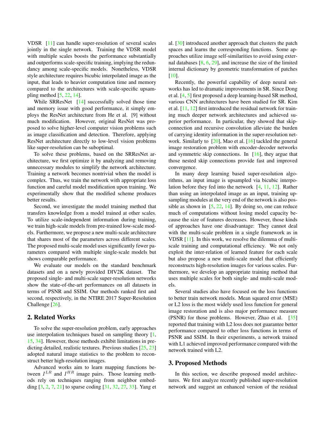
1 . Enhanced Deep Residual Networks for Single Image Super-Resolution Bee Lim Sanghyun Son Heewon Kim Seungjun Nah Kyoung Mu Lee Department of ECE, ASRI, Seoul National University, 08826, Seoul, Korea forestrainee@gmail.com, thstkdgus35@snu.ac.kr, ghimhw@gmail.com seungjun.nah@gmail.com, kyoungmu@snu.ac.kr arXiv:1707.02921v1 [cs.CV] 10 Jul 2017 Abstract Recent research on super-resolution has progressed with the development of deep convolutional neural networks (DCNN). In particular, residual learning techniques exhibit improved performance. In this paper, we develop an en- hanced deep super-resolution network (EDSR) with perfor- mance exceeding those of current state-of-the-art SR meth- HR ods. The significant performance improvement of our model (PSNR / SSIM) is due to optimization by removing unnecessary modules in conventional residual networks. The performance is further improved by expanding the model size while we stabilize the training procedure. We also propose a new multi-scale deep super-resolution system (MDSR) and training method, which can reconstruct high-resolution images of different upscaling factors in a single model. The proposed methods 0853 from DIV2K [26] Bicubic show superior performance over the state-of-the-art meth- (30.80 dB / 0.9537) ods on benchmark datasets and prove its excellence by win- ning the NTIRE2017 Super-Resolution Challenge [26]. 1. Introduction Image super-resolution (SR) problem, particularly sin- gle image super-resolution (SISR), has gained increasing VDSR [11] SRResNet [14] EDSR+ (Ours) research attention for decades. SISR aims to reconstruct (32.82 dB / 0.9623) (34.00 dB / 0.9679) (34.78 dB / 0.9708) a high-resolution image I SR from a single low-resolution image I LR . Generally, the relationship between I LR and Figure 1: ×4 Super-resolution result of our single-scale SR the original high-resolution image I HR can vary depending method (EDSR) compared with existing algorithms. on the situation. Many studies assume that I LR is a bicubic downsampled version of I HR , but other degrading factors such as blur, decimation, or noise can also be considered for ferent initialization and training techniques. Thus, carefully practical applications. designed model architecture and sophisticated optimization Recently, deep neural networks [11, 12, 14] provide sig- methods are essential in training the neural networks. nificantly improved performance in terms of peak signal-to- Second, most existing SR algorithms treat super- noise ratio (PSNR) in the SR problem. However, such net- resolution of different scale factors as independent prob- works exhibit limitations in terms of architecture optimality. lems without considering and utilizing mutual relationships First, the reconstruction performance of the neural network among different scales in SR. As such, those algorithms re- models is sensitive to minor architectural changes. Also, the quire many scale-specific networks that need to to be trained same model achieves different levels of performance by dif- independently to deal with various scales. Exceptionally, 1 

2 .VDSR [11] can handle super-resolution of several scales al. [30] introduced another approach that clusters the patch jointly in the single network. Training the VDSR model spaces and learns the corresponding functions. Some ap- with multiple scales boosts the performance substantially proaches utilize image self-similarities to avoid using exter- and outperforms scale-specific training, implying the redun- nal databases [8, 6, 29], and increase the size of the limited dancy among scale-specific models. Nonetheless, VDSR internal dictionary by geometric transformation of patches style architecture requires bicubic interpolated image as the [10]. input, that leads to heavier computation time and memory Recently, the powerful capability of deep neural net- compared to the architectures with scale-specific upsam- works has led to dramatic improvements in SR. Since Dong pling method [5, 22, 14]. et al. [4, 5] first proposed a deep learning-based SR method, While SRResNet [14] successfully solved those time various CNN architectures have been studied for SR. Kim and memory issue with good performance, it simply em- et al. [11, 12] first introduced the residual network for train- ploys the ResNet architecture from He et al. [9] without ing much deeper network architectures and achieved su- much modification. However, original ResNet was pro- perior performance. In particular, they showed that skip- posed to solve higher-level computer vision problems such connection and recursive convolution alleviate the burden as image classification and detection. Therefore, applying of carrying identity information in the super-resolution net- ResNet architecture directly to low-level vision problems work. Similarly to [20], Mao et al. [16] tackled the general like super-resolution can be suboptimal. image restoration problem with encoder-decoder networks To solve these problems, based on the SRResNet ar- and symmetric skip connections. In [16], they argue that chitecture, we first optimize it by analyzing and removing those nested skip connections provide fast and improved unnecessary modules to simplify the network architecture. convergence. Training a network becomes nontrivial when the model is In many deep learning based super-resolution algo- complex. Thus, we train the network with appropriate loss rithms, an input image is upsampled via bicubic interpo- function and careful model modification upon training. We lation before they fed into the network [4, 11, 12]. Rather experimentally show that the modified scheme produces than using an interpolated image as an input, training up- better results. sampling modules at the very end of the network is also pos- Second, we investigate the model training method that sible as shown in [5, 22, 14]. By doing so, one can reduce transfers knowledge from a model trained at other scales. much of computations without losing model capacity be- To utilize scale-independent information during training, cause the size of features decreases. However, those kinds we train high-scale models from pre-trained low-scale mod- of approaches have one disadvantage: They cannot deal els. Furthermore, we propose a new multi-scale architecture with the multi-scale problem in a single framework as in that shares most of the parameters across different scales. VDSR [11]. In this work, we resolve the dilemma of multi- The proposed multi-scale model uses significantly fewer pa- scale training and computational efficiency. We not only rameters compared with multiple single-scale models but exploit the inter-relation of learned feature for each scale shows comparable performance. but also propose a new multi-scale model that efficiently We evaluate our models on the standard benchmark reconstructs high-resolution images for various scales. Fur- datasets and on a newly provided DIV2K dataset. The thermore, we develop an appropriate training method that proposed single- and multi-scale super-resolution networks uses multiple scales for both single- and multi-scale mod- show the state-of-the-art performances on all datasets in els. terms of PSNR and SSIM. Our methods ranked first and Several studies also have focused on the loss functions second, respectively, in the NTIRE 2017 Super-Resolution to better train network models. Mean squared error (MSE) Challenge [26]. or L2 loss is the most widely used loss function for general image restoration and is also major performance measure 2. Related Works (PSNR) for those problems. However, Zhao et al. [35] reported that training with L2 loss does not guarantee better To solve the super-resolution problem, early approaches performance compared to other loss functions in terms of use interpolation techniques based on sampling theory [1, PSNR and SSIM. In their experiments, a network trained 15, 34]. However, those methods exhibit limitations in pre- with L1 achieved improved performance compared with the dicting detailed, realistic textures. Previous studies [25, 23] network trained with L2. adopted natural image statistics to the problem to recon- struct better high-resolution images. 3. Proposed Methods Advanced works aim to learn mapping functions be- tween I LR and I HR image pairs. Those learning meth- In this section, we describe proposed model architec- ods rely on techniques ranging from neighbor embed- tures. We first analyze recently published super-resolution ding [3, 2, 7, 21] to sparse coding [31, 32, 27, 33]. Yang et network and suggest an enhanced version of the residual 

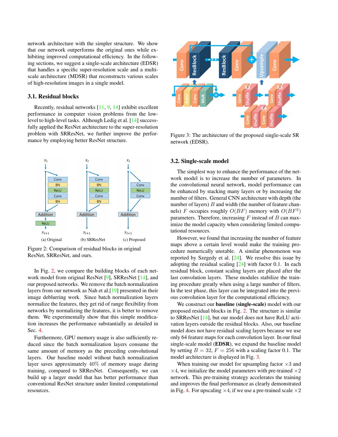
3 .network architecture with the simpler structure. We show that our network outperforms the original ones while ex- Upsample hibiting improved computational efficiency. In the follow- ResBlock ResBlock ••• Conv Conv Conv ing sections, we suggest a single-scale architecture (EDSR) that handles a specific super-resolution scale and a multi- scale architecture (MDSR) that reconstructs various scales of high-resolution images in a single model. X2 X3 Shuffle Shuffle ReLU 3.1. Residual blocks Conv Conv Conv Conv Mult Recently, residual networks [11, 9, 14] exhibit excellent X4 performance in computer vision problems from the low- Shuffle Shuffle Conv Conv level to high-level tasks. Although Ledig et al. [14] success- fully applied the ResNet architecture to the super-resolution problem with SRResNet, we further improve the perfor- Figure 3: The architecture of the proposed single-scale SR mance by employing better ResNet structure. network (EDSR). ResBlock 3.2. Single-scale model Conv (X2) X2 The simplest way to enhance the performance of the net- work model is to increase the number of parameters. In ResBlock ResBlock ResBlock the convolutional neural• • •network, model performance can Conv Conv Conv (X3) X3 be enhanced by stacking many layers or by increasing the number of filters. General CNN architecture with depth (the number of layers) B and width (the number of feature chan- nels) F occupies roughly O(BF ) memory with O(BF 2 ) ResBlock Conv (X4) parameters. Therefore, increasing F instead of B can max- X4 imize the model capacity when considering limited compu- tational resources. (a) Original (b) SRResNet (c) Proposed However, we found that increasing the number of feature maps above a certain level would make the training pro- Figure 2: Comparison of residual blocks in original cedure numerically unstable. A similar phenomenon was ResNet, SRResNet, and ours. reported by Szegedy et al. [24]. We resolve this issue by adopting the residual scaling [24] with factor 0.1. In each In Fig. 2, we compare the building blocks of each net- residual block, constant scaling layers are placed after the work model from original ResNet [9], SRResNet [14], and last convolution layers. These modules stabilize the train- our proposed networks. We remove the batch normalization ing procedure greatly when using a large number of filters. layers from our network as Nah et al.[19] presented in their In the test phase, this layer can be integrated into the previ- image deblurring work. Since batch normalization layers ous convolution layer for the computational efficiency. normalize the features, they get rid of range flexibility from We construct our baseline (single-scale) model with our networks by normalizing the features, it is better to remove proposed residual blocks in Fig. 2. The structure is similar them. We experimentally show that this simple modifica- to SRResNet [14], but our model does not have ReLU acti- tion increases the performance substantially as detailed in vation layers outside the residual blocks. Also, our baseline Sec. 4. model does not have residual scaling layers because we use Furthermore, GPU memory usage is also sufficiently re- only 64 feature maps for each convolution layer. In our final duced since the batch normalization layers consume the single-scale model (EDSR), we expand the baseline model same amount of memory as the preceding convolutional by setting B = 32, F = 256 with a scaling factor 0.1. The layers. Our baseline model without batch normalization model architecture is displayed in Fig. 3. layer saves approximately 40% of memory usage during When training our model for upsampling factor ×3 and training, compared to SRResNet. Consequently, we can ×4, we initialize the model parameters with pre-trained ×2 build up a larger model that has better performance than network. This pre-training strategy accelerates the training conventional ResNet structure under limited computational and improves the final performance as clearly demonstrated resources. in Fig. 4. For upscaling ×4, if we use a pre-trained scale ×2 

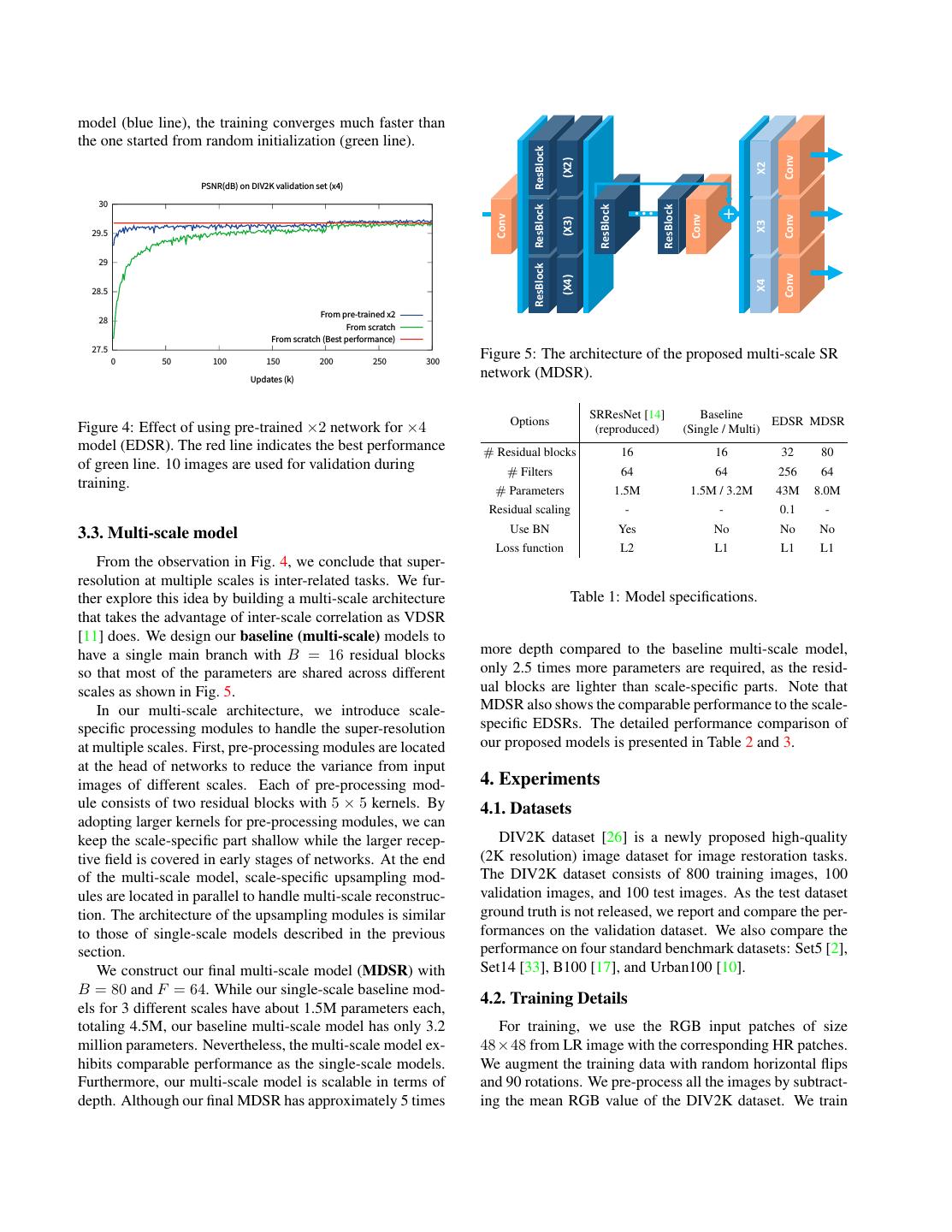
4 . X2 X3 Shuffle Shuffle ReLU Conv Conv Conv Conv Mult X4 Shuffle Shuffle Conv Conv model (blue line), the training converges much faster than the one started from random initialization (green line). ResBlock Conv (X2) X2 PSNR(dB) on DIV2K validation set (x4) 30 ResBlock ResBlock ResBlock ••• Conv Conv Conv (X3) X3 29.5 29 ResBlock Conv (X4) X4 28.5 From pre-trained x2 28 From scratch From scratch (Best performance) 27.5 0 50 100 150 200 250 300 Figure 5: The architecture of the proposed multi-scale SR Updates (k) network (MDSR). SRResNet [14] Baseline Figure 4: Effect of using pre-trained ×2 network for ×4 Options EDSR MDSR (reproduced) (Single / Multi) model (EDSR). The red line indicates the best performance # Residual blocks 16 16 32 80 of green line. 10 images are used for validation during # Filters 64 64 256 64 training. # Parameters 1.5M 1.5M / 3.2M 43M 8.0M Residual scaling - - 0.1 - 3.3. Multi-scale model Use BN Yes No No No Loss function L2 L1 L1 L1 From the observation in Fig. 4, we conclude that super- resolution at multiple scales is inter-related tasks. We fur- ther explore this idea by building a multi-scale architecture Table 1: Model specifications. that takes the advantage of inter-scale correlation as VDSR [11] does. We design our baseline (multi-scale) models to have a single main branch with B = 16 residual blocks more depth compared to the baseline multi-scale model, so that most of the parameters are shared across different only 2.5 times more parameters are required, as the resid- scales as shown in Fig. 5. ual blocks are lighter than scale-specific parts. Note that In our multi-scale architecture, we introduce scale- MDSR also shows the comparable performance to the scale- specific processing modules to handle the super-resolution specific EDSRs. The detailed performance comparison of at multiple scales. First, pre-processing modules are located our proposed models is presented in Table 2 and 3. at the head of networks to reduce the variance from input images of different scales. Each of pre-processing mod- 4. Experiments ule consists of two residual blocks with 5 × 5 kernels. By 4.1. Datasets adopting larger kernels for pre-processing modules, we can keep the scale-specific part shallow while the larger recep- DIV2K dataset [26] is a newly proposed high-quality tive field is covered in early stages of networks. At the end (2K resolution) image dataset for image restoration tasks. of the multi-scale model, scale-specific upsampling mod- The DIV2K dataset consists of 800 training images, 100 ules are located in parallel to handle multi-scale reconstruc- validation images, and 100 test images. As the test dataset tion. The architecture of the upsampling modules is similar ground truth is not released, we report and compare the per- to those of single-scale models described in the previous formances on the validation dataset. We also compare the section. performance on four standard benchmark datasets: Set5 [2], We construct our final multi-scale model (MDSR) with Set14 [33], B100 [17], and Urban100 [10]. B = 80 and F = 64. While our single-scale baseline mod- 4.2. Training Details els for 3 different scales have about 1.5M parameters each, totaling 4.5M, our baseline multi-scale model has only 3.2 For training, we use the RGB input patches of size million parameters. Nevertheless, the multi-scale model ex- 48×48 from LR image with the corresponding HR patches. hibits comparable performance as the single-scale models. We augment the training data with random horizontal flips Furthermore, our multi-scale model is scalable in terms of and 90 rotations. We pre-process all the images by subtract- depth. Although our final MDSR has approximately 5 times ing the mean RGB value of the DIV2K dataset. We train 

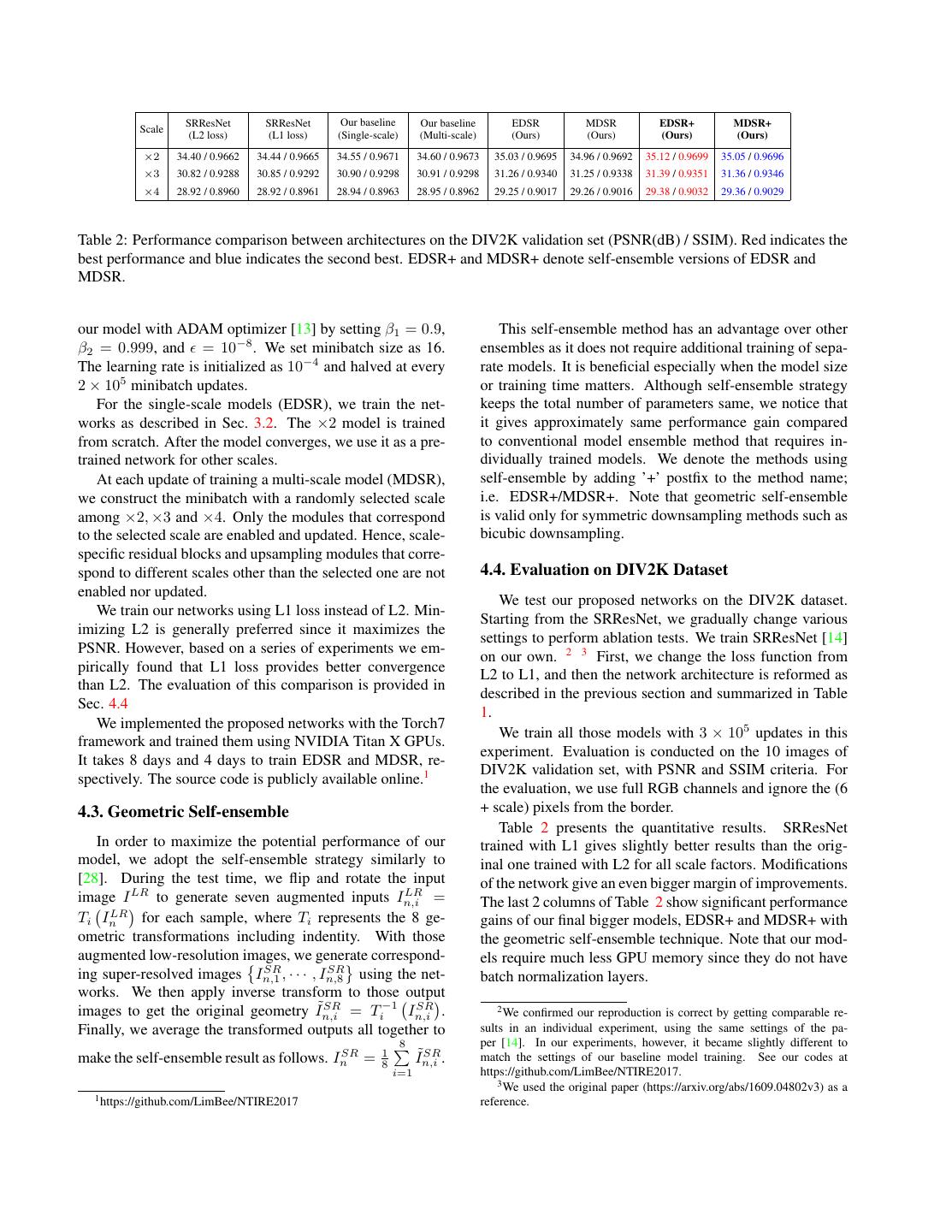
5 . SRResNet SRResNet Our baseline Our baseline EDSR MDSR EDSR+ MDSR+ Scale (L2 loss) (L1 loss) (Single-scale) (Multi-scale) (Ours) (Ours) (Ours) (Ours) ×2 34.40 / 0.9662 34.44 / 0.9665 34.55 / 0.9671 34.60 / 0.9673 35.03 / 0.9695 34.96 / 0.9692 35.12 / 0.9699 35.05 / 0.9696 ×3 30.82 / 0.9288 30.85 / 0.9292 30.90 / 0.9298 30.91 / 0.9298 31.26 / 0.9340 31.25 / 0.9338 31.39 / 0.9351 31.36 / 0.9346 ×4 28.92 / 0.8960 28.92 / 0.8961 28.94 / 0.8963 28.95 / 0.8962 29.25 / 0.9017 29.26 / 0.9016 29.38 / 0.9032 29.36 / 0.9029 Table 2: Performance comparison between architectures on the DIV2K validation set (PSNR(dB) / SSIM). Red indicates the best performance and blue indicates the second best. EDSR+ and MDSR+ denote self-ensemble versions of EDSR and MDSR. our model with ADAM optimizer [13] by setting β1 = 0.9, This self-ensemble method has an advantage over other β2 = 0.999, and = 10−8 . We set minibatch size as 16. ensembles as it does not require additional training of sepa- The learning rate is initialized as 10−4 and halved at every rate models. It is beneficial especially when the model size 2 × 105 minibatch updates. or training time matters. Although self-ensemble strategy For the single-scale models (EDSR), we train the net- keeps the total number of parameters same, we notice that works as described in Sec. 3.2. The ×2 model is trained it gives approximately same performance gain compared from scratch. After the model converges, we use it as a pre- to conventional model ensemble method that requires in- trained network for other scales. dividually trained models. We denote the methods using At each update of training a multi-scale model (MDSR), self-ensemble by adding ’+’ postfix to the method name; we construct the minibatch with a randomly selected scale i.e. EDSR+/MDSR+. Note that geometric self-ensemble among ×2, ×3 and ×4. Only the modules that correspond is valid only for symmetric downsampling methods such as to the selected scale are enabled and updated. Hence, scale- bicubic downsampling. specific residual blocks and upsampling modules that corre- spond to different scales other than the selected one are not 4.4. Evaluation on DIV2K Dataset enabled nor updated. We test our proposed networks on the DIV2K dataset. We train our networks using L1 loss instead of L2. Min- Starting from the SRResNet, we gradually change various imizing L2 is generally preferred since it maximizes the settings to perform ablation tests. We train SRResNet [14] PSNR. However, based on a series of experiments we em- on our own. 2 3 First, we change the loss function from pirically found that L1 loss provides better convergence L2 to L1, and then the network architecture is reformed as than L2. The evaluation of this comparison is provided in described in the previous section and summarized in Table Sec. 4.4 1. We implemented the proposed networks with the Torch7 We train all those models with 3 × 105 updates in this framework and trained them using NVIDIA Titan X GPUs. experiment. Evaluation is conducted on the 10 images of It takes 8 days and 4 days to train EDSR and MDSR, re- DIV2K validation set, with PSNR and SSIM criteria. For spectively. The source code is publicly available online.1 the evaluation, we use full RGB channels and ignore the (6 4.3. Geometric Self-ensemble + scale) pixels from the border. Table 2 presents the quantitative results. SRResNet In order to maximize the potential performance of our trained with L1 gives slightly better results than the orig- model, we adopt the self-ensemble strategy similarly to inal one trained with L2 for all scale factors. Modifications [28]. During the test time, we flip and rotate the input of the network give an even bigger margin of improvements. image I LR to generate seven augmented inputs In,i LR = The last 2 columns of Table 2 show significant performance LR Ti In for each sample, where Ti represents the 8 ge- gains of our final bigger models, EDSR+ and MDSR+ with ometric transformations including indentity. With those the geometric self-ensemble technique. Note that our mod- augmented low-resolution images, we generate correspond- els require much less GPU memory since they do not have SR SR ing super-resolved images In,1 , · · · , In,8 using the net- batch normalization layers. works. We then apply inverse transform to those output images to get the original geometry I˜n,i SR = Ti−1 In,i SR . 2 We confirmed our reproduction is correct by getting comparable re- Finally, we average the transformed outputs all together to sults in an individual experiment, using the same settings of the pa- 8 per [14]. In our experiments, however, it became slightly different to make the self-ensemble result as follows. InSR = 1 8 I˜n,i SR . match the settings of our baseline model training. See our codes at i=1 https://github.com/LimBee/NTIRE2017. 3 We used the original paper (https://arxiv.org/abs/1609.04802v3) as a 1 https://github.com/LimBee/NTIRE2017 reference. 

6 . HR Bicubic A+ [27] SRCNN [4] (PSNR / SSIM) (21.41 dB / 0.4810) (22.21 dB / 0.5408) (22.33 dB / 0.5461) img034 from Urban100 [10] VDSR [11] SRResNet [14] EDSR+ (Ours) MDSR+ (Ours) (22.62 dB / 0.5657) (23.14 dB / 0.5891) (23.48 dB / 0.6048) (23.46 dB / 0.6039) HR Bicubic A+ [27] SRCNN [4] (PSNR / SSIM) (19.82 dB / 0.6471) (20.43 dB 0.7145) (20.61 dB / 0.7218) img062 from Urban100 [10] VDSR [11] SRResNet [14] EDSR+ (Ours) MDSR+ (Ours) (20.75 dB / 0.7504) (21.70 dB / 0.8054) (22.70 dB / 0.8537) (22.66 dB / 0.8508) HR Bicubic A+ [27] SRCNN [4] (PSNR / SSIM) (22.66 dB / 0.8025) (23.10 dB / 0.8251) (23.14 dB / 0.8280) 0869 from DIV2K [26] VDSR [11] SRResNet [14] EDSR+ (Ours) MDSR+ (Ours) (23.36 dB / 0.8365) (23.71 dB / 0.8485) (23.89 dB / 0.8563) (23.90 dB / 0.8558) Figure 6: Qualitative comparison of our models with other works on ×4 super-resolution. 

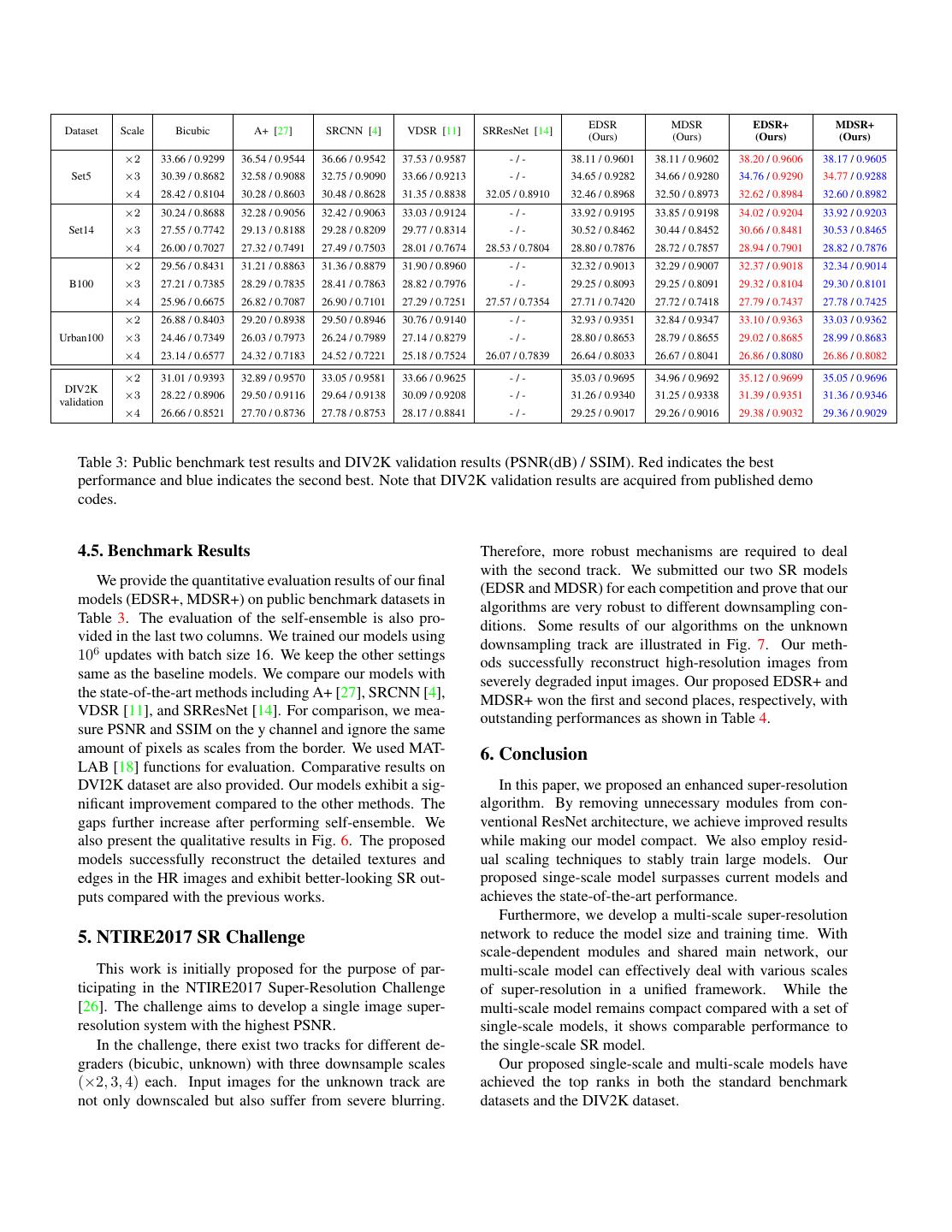
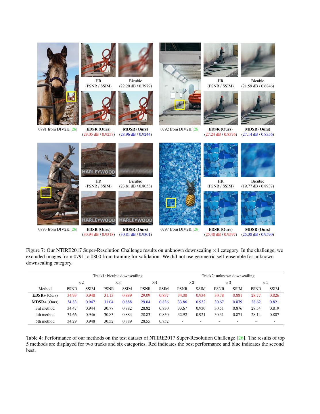
7 . EDSR MDSR EDSR+ MDSR+ Dataset Scale Bicubic A+ [27] SRCNN [4] VDSR [11] SRResNet [14] (Ours) (Ours) (Ours) (Ours) ×2 33.66 / 0.9299 36.54 / 0.9544 36.66 / 0.9542 37.53 / 0.9587 -/- 38.11 / 0.9601 38.11 / 0.9602 38.20 / 0.9606 38.17 / 0.9605 Set5 ×3 30.39 / 0.8682 32.58 / 0.9088 32.75 / 0.9090 33.66 / 0.9213 -/- 34.65 / 0.9282 34.66 / 0.9280 34.76 / 0.9290 34.77 / 0.9288 ×4 28.42 / 0.8104 30.28 / 0.8603 30.48 / 0.8628 31.35 / 0.8838 32.05 / 0.8910 32.46 / 0.8968 32.50 / 0.8973 32.62 / 0.8984 32.60 / 0.8982 ×2 30.24 / 0.8688 32.28 / 0.9056 32.42 / 0.9063 33.03 / 0.9124 -/- 33.92 / 0.9195 33.85 / 0.9198 34.02 / 0.9204 33.92 / 0.9203 Set14 ×3 27.55 / 0.7742 29.13 / 0.8188 29.28 / 0.8209 29.77 / 0.8314 -/- 30.52 / 0.8462 30.44 / 0.8452 30.66 / 0.8481 30.53 / 0.8465 ×4 26.00 / 0.7027 27.32 / 0.7491 27.49 / 0.7503 28.01 / 0.7674 28.53 / 0.7804 28.80 / 0.7876 28.72 / 0.7857 28.94 / 0.7901 28.82 / 0.7876 ×2 29.56 / 0.8431 31.21 / 0.8863 31.36 / 0.8879 31.90 / 0.8960 -/- 32.32 / 0.9013 32.29 / 0.9007 32.37 / 0.9018 32.34 / 0.9014 B100 ×3 27.21 / 0.7385 28.29 / 0.7835 28.41 / 0.7863 28.82 / 0.7976 -/- 29.25 / 0.8093 29.25 / 0.8091 29.32 / 0.8104 29.30 / 0.8101 ×4 25.96 / 0.6675 26.82 / 0.7087 26.90 / 0.7101 27.29 / 0.7251 27.57 / 0.7354 27.71 / 0.7420 27.72 / 0.7418 27.79 / 0.7437 27.78 / 0.7425 ×2 26.88 / 0.8403 29.20 / 0.8938 29.50 / 0.8946 30.76 / 0.9140 -/- 32.93 / 0.9351 32.84 / 0.9347 33.10 / 0.9363 33.03 / 0.9362 Urban100 ×3 24.46 / 0.7349 26.03 / 0.7973 26.24 / 0.7989 27.14 / 0.8279 -/- 28.80 / 0.8653 28.79 / 0.8655 29.02 / 0.8685 28.99 / 0.8683 ×4 23.14 / 0.6577 24.32 / 0.7183 24.52 / 0.7221 25.18 / 0.7524 26.07 / 0.7839 26.64 / 0.8033 26.67 / 0.8041 26.86 / 0.8080 26.86 / 0.8082 ×2 31.01 / 0.9393 32.89 / 0.9570 33.05 / 0.9581 33.66 / 0.9625 -/- 35.03 / 0.9695 34.96 / 0.9692 35.12 / 0.9699 35.05 / 0.9696 DIV2K ×3 28.22 / 0.8906 29.50 / 0.9116 29.64 / 0.9138 30.09 / 0.9208 -/- 31.26 / 0.9340 31.25 / 0.9338 31.39 / 0.9351 31.36 / 0.9346 validation ×4 26.66 / 0.8521 27.70 / 0.8736 27.78 / 0.8753 28.17 / 0.8841 -/- 29.25 / 0.9017 29.26 / 0.9016 29.38 / 0.9032 29.36 / 0.9029 Table 3: Public benchmark test results and DIV2K validation results (PSNR(dB) / SSIM). Red indicates the best performance and blue indicates the second best. Note that DIV2K validation results are acquired from published demo codes. 4.5. Benchmark Results Therefore, more robust mechanisms are required to deal with the second track. We submitted our two SR models We provide the quantitative evaluation results of our final (EDSR and MDSR) for each competition and prove that our models (EDSR+, MDSR+) on public benchmark datasets in algorithms are very robust to different downsampling con- Table 3. The evaluation of the self-ensemble is also pro- ditions. Some results of our algorithms on the unknown vided in the last two columns. We trained our models using downsampling track are illustrated in Fig. 7. Our meth- 106 updates with batch size 16. We keep the other settings ods successfully reconstruct high-resolution images from same as the baseline models. We compare our models with severely degraded input images. Our proposed EDSR+ and the state-of-the-art methods including A+ [27], SRCNN [4], MDSR+ won the first and second places, respectively, with VDSR [11], and SRResNet [14]. For comparison, we mea- outstanding performances as shown in Table 4. sure PSNR and SSIM on the y channel and ignore the same amount of pixels as scales from the border. We used MAT- 6. Conclusion LAB [18] functions for evaluation. Comparative results on DVI2K dataset are also provided. Our models exhibit a sig- In this paper, we proposed an enhanced super-resolution nificant improvement compared to the other methods. The algorithm. By removing unnecessary modules from con- gaps further increase after performing self-ensemble. We ventional ResNet architecture, we achieve improved results also present the qualitative results in Fig. 6. The proposed while making our model compact. We also employ resid- models successfully reconstruct the detailed textures and ual scaling techniques to stably train large models. Our edges in the HR images and exhibit better-looking SR out- proposed singe-scale model surpasses current models and puts compared with the previous works. achieves the state-of-the-art performance. Furthermore, we develop a multi-scale super-resolution 5. NTIRE2017 SR Challenge network to reduce the model size and training time. With scale-dependent modules and shared main network, our This work is initially proposed for the purpose of par- multi-scale model can effectively deal with various scales ticipating in the NTIRE2017 Super-Resolution Challenge of super-resolution in a unified framework. While the [26]. The challenge aims to develop a single image super- multi-scale model remains compact compared with a set of resolution system with the highest PSNR. single-scale models, it shows comparable performance to In the challenge, there exist two tracks for different de- the single-scale SR model. graders (bicubic, unknown) with three downsample scales Our proposed single-scale and multi-scale models have (×2, 3, 4) each. Input images for the unknown track are achieved the top ranks in both the standard benchmark not only downscaled but also suffer from severe blurring. datasets and the DIV2K dataset. 

8 . HR Bicubic HR Bicubic (PSNR / SSIM) (22.20 dB / 0.7979) (PSNR / SSIM) (21.59 dB / 0.6846) 0791 from DIV2K [26] EDSR (Ours) MDSR (Ours) 0792 from DIV2K [26] EDSR (Ours) MDSR (Ours) (29.05 dB / 0.9257) (28.96 dB / 0.9244) (27.24 dB / 0.8376) (27.14 dB / 0.8356) HR Bicubic HR Bicubic (PSNR / SSIM) (23.81 dB / 0.8053) (PSNR / SSIM) (19.77 dB / 0.8937) 0793 from DIV2K [26] EDSR (Ours) MDSR (Ours) 0797 from DIV2K [26] EDSR (Ours) MDSR (Ours) (30.94 dB / 0.9318) (30.81 dB / 0.9301) (25.48 dB / 0.9597) (25.38 dB / 0.9590) Figure 7: Our NTIRE2017 Super-Resolution Challenge results on unknown downscaling ×4 category. In the challenge, we excluded images from 0791 to 0800 from training for validation. We did not use geometric self-ensemble for unknown downscaling category. Track1: bicubic downscailing Track2: unknown downscailing ×2 ×3 ×4 ×2 ×3 ×4 Method PSNR SSIM PSNR SSIM PSNR SSIM PSNR SSIM PSNR SSIM PSNR SSIM EDSR+ (Ours) 34.93 0.948 31.13 0.889 29.09 0.837 34.00 0.934 30.78 0.881 28.77 0.826 MDSR+ (Ours) 34.83 0.947 31.04 0.888 29.04 0.836 33.86 0.932 30.67 0.879 28.62 0.821 3rd method 34.47 0.944 30.77 0.882 28.82 0.830 33.67 0.930 30.51 0.876 28.54 0.819 4th method 34.66 0.946 30.83 0.884 28.83 0.830 32.92 0.921 30.31 0.871 28.14 0.807 5th method 34.29 0.948 30.52 0.889 28.55 0.752 - - - - - - Table 4: Performance of our methods on the test dataset of NTIRE2017 Super-Resolution Challenge [26]. The results of top 5 methods are displayed for two tracks and six categories. Red indicates the best performance and blue indicates the second best. 

9 .References [21] S. T. Roweis and L. K. Saul. Nonlinear dimensionality reduc- tion by locally linear embedding. Science, 290(5500):2323– [1] J. Allebach and P. W. Wong. Edge-directed interpolation. In 2326, 2000. 2 ICIP 1996. 2 [22] W. Shi, J. Caballero, F. Husz´ar, J. Totz, A. P. Aitken, [2] M. Bevilacqua, A. Roumy, C. Guillemot, and M. L. Alberi- R. Bishop, D. Rueckert, and Z. Wang. Real-time single im- Morel. Low-complexity single-image super-resolution based age and video super-resolution using an efficient sub-pixel on nonnegative neighbor embedding. In BMVC 2012. 2, 4 convolutional neural network. In CVPR 2016. 2 [3] H. Chang, D.-Y. Yeung, and Y. Xiong. Super-resolution [23] J. Sun, Z. Xu, and H.-Y. Shum. Image super-resolution using through neighbor embedding. In CVPR 2004. 2 gradient profile prior. In CVPR 2008. 2 [4] C. Dong, C. C. Loy, K. He, and X. Tang. Learning a deep [24] C. Szegedy, S. Ioffe, V. Vanhoucke, and A. Alemi. Inception- convolutional network for image super-resolution. In ECCV v4, inception-resnet and the impact of residual connections 2014. 2, 6, 7 on learning. arXiv:1602.07261, 2016. 3 [5] C. Dong, C. C. Loy, and X. Tang. Accelerating the super- [25] Y.-W. Tai, S. Liu, M. S. Brown, and S. Lin. Super resolution resolution convolutional neural network. In ECCV 2016. 2 using edge prior and single image detail synthesis. In CVPR [6] G. Freedman and R. Fattal. Image and video upscaling from 2010. 2 local self-examples. ACM Transactions on Graphics (TOG), 30(2):12, 2011. 2 [26] R. Timofte, E. Agustsson, L. Van Gool, M.-H. Yang, L. Zhang, et al. Ntire 2017 challenge on single image super- [7] X. Gao, K. Zhang, D. Tao, and X. Li. Image super-resolution resolution: Methods and results. In CVPR 2017 Workshops. with sparse neighbor embedding. IEEE Transactions on Im- 1, 2, 4, 6, 7, 8 age Processing, 21(7):3194–3205, 2012. 2 [8] D. Glasner, S. Bagon, and M. Irani. Super-resolution from a [27] R. Timofte, V. De Smet, and L. Van Gool. A+: Adjusted single image. In ICCV 2009. 2 anchored neighborhood regression for fast super-resolution. In ACCV 2014. 2, 6, 7 [9] K. He, X. Zhang, S. Ren, and J. Sun. Deep residual learning for image recognition. In CVPR 2016. 3 [28] R. Timofte, R. Rothe, and L. Van Gool. Seven ways to [10] J.-B. Huang, A. Singh, and N. Ahuja. Single image super- improve example-based single image super resolution. In resolution from transformed self-exemplars. In CVPR 2015. CVPR 2016. 5 2, 4, 6 [29] Z. Wang, Y. Yang, Z. Wang, S. Chang, J. Yang, and T. S. [11] J. Kim, J. Kwon Lee, and K. M. Lee. Accurate image super- Huang. Learning super-resolution jointly from external and resolution using very deep convolutional networks. In CVPR internal examples. IEEE Transactions on Image Processing, 2016. 1, 2, 3, 4, 6, 7 24(11):4359–4371, 2015. 2 [12] J. Kim, J. Kwon Lee, and K. M. Lee. Deeply-recursive [30] C.-Y. Yang and M.-H. Yang. Fast direct super-resolution by convolutional network for image super-resolution. In CVPR simple functions. In ICCV 2013. 2 2016. 1, 2 [31] J. Yang, Z. Wang, Z. Lin, S. Cohen, and T. Huang. Coupled [13] D. Kingma and J. Ba. Adam: A method for stochastic opti- dictionary training for image super-resolution. IEEE Trans- mization. In ICLR 2014. 5 actions on Image Processing, 21(8):3467–3478, 2012. 2 [14] C. Ledig, L. Theis, F. Husz´ar, J. Caballero, A. Cunningham, [32] J. Yang, J. Wright, T. S. Huang, and Y. Ma. Image super- A. Acosta, A. Aitken, A. Tejani, J. Totz, Z. Wang, et al. resolution via sparse representation. IEEE Transactions on Photo-realistic single image super-resolution using a gener- Image Processing, 19(11):2861–2873, 2010. 2 ative adversarial network. arXiv:1609.04802, 2016. 1, 2, 3, [33] R. Zeyde, M. Elad, and M. Protter. On single image scale-up 4, 5, 6, 7 using sparse-representations. In Proceedings of the Interna- [15] X. Li and M. T. Orchard. New edge-directed interpolation. tional Conference on Curves and Surfaces, 2010. 2, 4 IEEE Transactions on Image Processing, 10(10):1521–1527, [34] L. Zhang and X. Wu. An edge-guided image interpolation al- 2001. 2 gorithm via directional filtering and data fusion. IEEE Trans- [16] X. Mao, C. Shen, and Y.-B. Yang. Image restoration us- actions on Image Processing, 15(8):2226–2238, 2006. 2 ing very deep convolutional encoder-decoder networks with [35] H. Zhao, O. Gallo, I. Frosio, and J. Kautz. Loss functions for symmetric skip connections. In NIPS 2016. 2 neural networks for image processing. arXiv:1511.08861, [17] D. Martin, C. Fowlkes, D. Tal, and J. Malik. A database 2015. 2 of human segmented natural images and its application to evaluating segmentation algorithms and measuring ecologi- cal statistics. In ICCV 2001. 4 [18] MATLAB. version 9.1.0 (R2016b). The MathWorks Inc., Natick, Massachusetts, 2016. 7 [19] S. Nah, T. H. Kim, and K. M. Lee. Deep multi-scale convolutional neural network for dynamic scene deblurring. arXiv:1612.02177, 2016. 3 [20] O. Ronneberger, P. Fischer, and T. Brox. U-net: Convolu- tional networks for biomedical image segmentation. In MIC- CAI 2015. 2