Adversarial Variational Bayes

1 . Adversarial Variational Bayes: Unifying Variational Autoencoders and Generative Adversarial Networks Lars Mescheder 1 Sebastian Nowozin 2 Andreas Geiger 1 3 Abstract Variational Autoencoders (VAEs) are expressive f arXiv:1701.04722v4 [cs.LG] 11 Jun 2018 latent variable models that can be used to learn complex probability distributions from training data. However, the quality of the resulting model crucially relies on the expressiveness of the in- ference model. We introduce Adversarial Vari- Figure 1. We propose a method which enables neural samplers ational Bayes (AVB), a technique for training with intractable density for Variational Bayes and as inference Variational Autoencoders with arbitrarily expres- models for learning latent variable models. This toy exam- sive inference models. We achieve this by in- ple demonstrates our method’s ability to accurately approximate troducing an auxiliary discriminative network complex posterior distributions like the one shown on the right. that allows to rephrase the maximum-likelihood- problem as a two-player game, hence establish- more powerful. While many model classes such as Pixel- ing a principled connection between VAEs and RNNs (van den Oord et al., 2016b), PixelCNNs (van den Generative Adversarial Networks (GANs). We Oord et al., 2016a), real NVP (Dinh et al., 2016) and Plug show that in the nonparametric limit our method & Play generative networks (Nguyen et al., 2016) have yields an exact maximum-likelihood assignment been introduced and studied, the two most prominent ones for the parameters of the generative model, as are Variational Autoencoders (VAEs) (Kingma & Welling, well as the exact posterior distribution over the 2013; Rezende et al., 2014) and Generative Adversarial latent variables given an observation. Contrary Networks (GANs) (Goodfellow et al., 2014). to competing approaches which combine VAEs with GANs, our approach has a clear theoretical Both VAEs and GANs come with their own advantages justification, retains most advantages of standard and disadvantages: while GANs generally yield visually Variational Autoencoders and is easy to imple- sharper results when applied to learning a representation ment. of natural images, VAEs are attractive because they natu- rally yield both a generative model and an inference model. Moreover, it was reported, that VAEs often lead to better 1. Introduction log-likelihoods (Wu et al., 2016). The recently introduced BiGANs (Donahue et al., 2016; Dumoulin et al., 2016) add Generative models in machine learning are models that can an inference model to GANs. However, it was observed be trained on an unlabeled dataset and are capable of gener- that the reconstruction results often only vaguely resemble ating new data points after training is completed. As gen- the input and often do so only semantically and not in terms erating new content requires a good understanding of the of pixel values. training data at hand, such models are often regarded as a key ingredient to unsupervised learning. The failure of VAEs to generate sharp images is often at- tributed to the fact that the inference models used during In recent years, generative models have become more and training are usually not expressive enough to capture the 1 Autonomous Vision Group, MPI T¨ubingen 2 Microsoft true posterior distribution. Indeed, recent work shows that Research Cambridge 3 Computer Vision and Geometry using more expressive model classes can lead to substan- Group, ETH Z¨urich. Correspondence to: Lars Mescheder tially better results (Kingma et al., 2016), both visually <lars.mescheder@tuebingen.mpg.de>. and in terms of log-likelihood bounds. Recent work (Chen Proceedings of the 34 th International Conference on Machine et al., 2016) also suggests that highly expressive inference Learning, Sydney, Australia, PMLR 70, 2017. Copyright 2017 models are essential in presence of a strong decoder to al- by the author(s). low the model to make use of the latent space at all. 

2 . Adversarial Variational Bayes In this paper, we present Adversarial Variational Bayes x (AVB) 1 , a technique for training Variational Autoencoders x 1 with arbitrarily flexible inference models parameterized by f 1 neural networks. We can show that in the nonparametric f limit we obtain a maximum-likelihood assignment for the +/∗ generative model together with the correct posterior distri- Encoder z Encoder z bution. While there were some attempts at combining VAEs and g 2 g 2 GANs (Makhzani et al., 2015; Larsen et al., 2015), most +/∗ +/∗ of these attempts are not motivated from a maximum- likelihood point of view and therefore usually do not lead x x to maximum-likelihood assignments. For example, in Ad- Decoder Decoder versarial Autoencoders (AAEs) (Makhzani et al., 2015) the (a) Standard VAE (b) Our model Kullback-Leibler regularization term that appears in the training objective for VAEs is replaced with an adversarial Figure 2. Schematic comparison of a standard VAE and a VAE loss that encourages the aggregated posterior to be close to with black-box inference model, where 1 and 2 denote samples the prior over the latent variables. Even though AAEs do from some noise distribution. While more complicated inference not maximize a lower bound to the maximum-likelihood models for Variational Autoencoders are possible, they are usually objective, we show in Section 6.2 that AAEs can be in- not as flexible as our black-box approach. terpreted as an approximation to our approach, thereby es- of the generative model. tablishing a connection of AAEs to maximum-likelihood • We empirically demonstrate that our model is able learning. to learn rich posterior distributions and show that the Outside the context of generative models, AVB yields a model is able to generate compelling samples for com- new method for performing Variational Bayes (VB) with plex data sets. neural samplers. This is illustrated in Figure 1, where we used AVB to train a neural network to sample from a non- 2. Background trival unnormalized probability density. This allows to ac- curately approximate the posterior distribution of a prob- As our model is an extension of Variational Autoencoders abilistic model, e.g. for Bayesian parameter estimation. (VAEs) (Kingma & Welling, 2013; Rezende et al., 2014), The only other variational methods we are aware of that we start with a brief review of VAEs. can deal with such expressive inference models are based VAEs are specified by a parametric generative model pθ (x | on Stein Discrepancy (Ranganath et al., 2016; Liu & Feng, z) of the visible variables given the latent variables, a prior 2016). However, those methods usually do not directly tar- p(z) over the latent variables and an approximate inference get the reverse Kullback-Leibler-Divergence and can there- model qφ (z | x) over the latent variables given the visible fore not be used to approximate the variational lower bound variables. It can be shown that for learning a latent variable model. Our contributions are as follows: log pθ (x) ≥ −KL(qφ (z | x), p(z)) • We enable the usage of arbitrarily complex inference + Eqφ (z|x) log pθ (x | z). (2.1) models for Variational Autoencoders using adversarial The right hand side of (2.1) is called the variational lower training. bound or evidence lower bound (ELBO). If there is φ such • We give theoretical insights into our method, show- that qφ (z | x) = pθ (z | x), we would have ing that in the nonparametric limit our method recov- ers the true posterior distribution as well as a true log pθ (x) = max −KL(qφ (z | x), p(z)) maximum-likelihood assignment for the parameters φ 1 Concurrently to our work, several researchers have de- + Eqφ (z|x) log pθ (x | z). (2.2) scribed similar ideas. Some ideas of this paper were described independently by Husz´ar in a blog post on http://www. However, in general this is not true, so that we only have inference.vc and in Husz´ar (2017). The idea to use adversar- an inequality in (2.2). ial training to improve the encoder network was also suggested by Goodfellow in an exploratory talk he gave at NIPS 2016 and by Li When performing maximum-likelihood training, our goal & Liu (2016). A similar idea was also mentioned by Karaletsos is to optimize the marginal log-likelihood (2016) in the context of message passing in graphical models. EpD (x) log pθ (x), (2.3) 

3 . Adversarial Variational Bayes where pD is the data distribution. Unfortunately, com- The idea of our approach is to circumvent this problem by puting log pθ (x) requires marginalizing out z in pθ (x, z) implicitly representing the term which is usually intractable. Variational Bayes uses in- equality (2.1) to rephrase the intractable problem of opti- log p(z) − log qφ (z | x) (3.2) mizing (2.3) into as the optimal value of an additional real-valued discrimi- native network T (x, z) that we introduce to the problem. max max EpD (x) −KL(qφ (z | x), p(z)) More specifically, consider the following objective for the θ φ discriminator T (x, z) for a given qφ (x | z): + Eqφ (z|x) log pθ (x | z) . (2.4) max EpD (x) Eqφ (z|x) log σ(T (x, z)) T Due to inequality (2.1), we still optimize a lower bound to the true maximum-likelihood objective (2.3). + EpD (x) Ep(z) log (1 − σ(T (x, z))) . (3.3) Naturally, the quality of this lower bound depends on the Here, σ(t) := (1 + e−t )−1 denotes the sigmoid-function. expressiveness of the inference model qφ (z | x). Usually, Intuitively, T (x, z) tries to distinguish pairs (x, z) that were qφ (z | x) is taken to be a Gaussian distribution with diago- sampled independently using the distribution pD (x)p(z) nal covariance matrix whose mean and variance vectors are from those that were sampled using the current inference parameterized by neural networks with x as input (Kingma model, i.e., using pD (x)qφ (z | x). & Welling, 2013; Rezende et al., 2014). While this model To simplify the theoretical analysis, we assume that the is very flexible in its dependence on x, its dependence on model T (x, z) is flexible enough to represent any func- z is very restrictive, potentially limiting the quality of the tion of the two variables x and z. This assumption is often resulting generative model. Indeed, it was observed that referred to as the nonparametric limit (Goodfellow et al., applying standard Variational Autoencoders to natural im- 2014) and is justified by the fact that deep neural networks ages often results in blurry images (Larsen et al., 2015). are universal function approximators (Hornik et al., 1989). As it turns out, the optimal discriminator T ∗ (x, z) accord- 3. Method ing to the objective in (3.3) is given by the negative of (3.2). In this work we show how we can instead use a black-box inference model qφ (z | x) and use adversarial training to Proposition 1. For pθ (x | z) and qφ (z | x) fixed, the opti- obtain an approximate maximum likelihood assignment θ∗ mal discriminator T ∗ according to the objective in (3.3) is to θ and a close approximation qφ∗ (z | x) to the true pos- given by terior pθ∗ (z | x). This is visualized in Figure 2: on the left hand side the structure of a typical VAE is shown. The right T ∗ (x, z) = log qφ (z | x) − log p(z). (3.4) hand side shows our flexible black-box inference model. In contrast to a VAE with Gaussian inference model, we in- Proof. The proof is analogous to the proof of Proposition clude the noise 1 as additional input to the inference model 1 in Goodfellow et al. (2014). See the Supplementary Ma- instead of adding it at the very end, thereby allowing the in- terial ference network to learn complex probability distributions. for details. Together with (3.1), Proposition 1 allows us to write the 3.1. Derivation optimization objective in (2.4) as To derive our method, we rewrite the optimization problem max EpD (x) Eqφ (z|x) − T ∗ (x, z) + log pθ (x | z) , (3.5) in (2.4) as θ,φ where T ∗ (x, z) is defined as the function that maximizes max max EpD (x) Eqφ (z|x) log p(z) (3.3). θ φ − log qφ (z | x) + log pθ (x | z) . (3.1) To optimize (3.5), we need to calculate the gradients of (3.5) with respect to θ and φ. While taking the gradient When we have an explicit representation of qφ (z | x) such with respect to θ is straightforward, taking the gradient with as a Gaussian parameterized by a neural network, (3.1) can respect to φ is complicated by the fact that we have defined be optimized using the reparameterization trick (Kingma & T ∗ (x, z) indirectly as the solution of an auxiliary optimiza- Welling, 2013; Rezende & Mohamed, 2015) and stochastic tion problem which itself depends on φ. However, the fol- gradient descent. Unfortunately, this is not the case when lowing Proposition shows that taking the gradient with re- we define qφ (z | x) by a black-box procedure as illustrated spect to the explicit occurrence of φ in T ∗ (x, z) is not nec- in Figure 2b. essary: 

4 . Adversarial Variational Bayes Algorithm 1 Adversarial Variational Bayes (AVB) algorithm converges, any fix point of this algorithm yields 1: i ← 0 a stationary point of the objective in (2.4). 2: while not converged do Note that optimizing (3.5) with respect to φ while keep- 3: Sample {x(1) , . . . , x(m) } from data distrib. pD (x) ing θ and T fixed makes the encoder network collapse to 4: Sample {z (1) , . . . , z (m) } from prior p(z) a deterministic function. This is also a common problem 5: Sample { (1) , . . . , (m) } from N (0, 1) for regular GANs (Radford et al., 2015). It is therefore 6: Compute θ-gradient (eq. 3.7): crucial to keep the discriminative T network close to op- 1 m gθ ← m k=1 ∇θ log pθ x(k) | zφ x(k) , (k) timality while optimizing (3.5). A variant of Algorithm 1 therefore performs several SGD-updates for the adversary 7: Compute φ-gradient (eq. 3.7): for one SGD-update of the generative model. However, 1 m gφ ← m ∇φ −Tψ x(k) , zφ (x(k) , (k) ) k=1 throughout our experiments we use the simple 1-step ver- + log pθ x(k) | zφ (x(k) , (k) ) sion of AVB unless stated otherwise. 8: Compute ψ-gradient (eq. 3.3) : 1 m 3.3. Theoretical results gψ ← m k=1 ∇ψ log σ(Tψ (x(k) , zφ (x(k) , (k) ))) In Sections 3.1 we derived AVB as a way of performing + log 1 − σ(Tψ (x(k) , z (k) ) stochastic gradient descent on the variational lower bound in (2.4). In this section, we analyze the properties of Algo- 9: Perform SGD-updates for θ, φ and ψ: rithm 1 from a game theoretical point of view. θ ← θ + hi gθ , φ ← φ + hi gφ , ψ ← ψ + hi gψ 10: i←i+1 As the next proposition shows, global Nash-equilibria of 11: end while Algorithm 1 yield global optima of the objective in (2.4): Proposition 3. Assume that T can represent any function of two variables. If (θ∗ , φ∗ , T ∗ ) defines a Nash-equilibrium Proposition 2. We have of the two-player game defined by (3.3) and (3.7), Eqφ (z|x) (∇φ T ∗ (x, z)) = 0. (3.6) then T ∗ (x, z) = log qφ∗ (z | x) − log p(z) (3.8) Proof. The proof can be found in the Supplementary Ma- and (θ∗ , φ∗ ) is a global optimum of the variational lower terial. bound in (2.4). Using the reparameterization trick (Kingma & Welling, 2013; Rezende et al., 2014), (3.5) can be rewritten in the Proof. The proof can be found in the Supplementary Ma- form terial. max EpD (x) E − T ∗ (x, zφ (x, )) Our parameterization of qφ (z | x) as a neural network al- θ,φ lows qφ (z | x) to represent almost any probability density + log pθ (x | zφ (x, )) (3.7) on the latent space. This motivates Corollary 4. Assume that T can represent any function of for a suitable function zφ (x, ). Together with Proposition two variables and qφ (z | x) can represent any probability 1, (3.7) allows us to take unbiased estimates of the gradients density on the latent space. If (θ∗ , φ∗ , T ∗ ) defines a Nash- of (3.5) with respect to φ and θ. equilibrium for the game defined by (3.3) and (3.7), then 3.2. Algorithm 1. θ∗ is a maximum-likelihood assignment In theory, Propositions 1 and 2 allow us to apply Stochastic Gradient Descent (SGD) directly to the objective in (2.4). 2. qφ∗ (z | x) is equal to the true posterior pθ∗ (z | x) However, this requires keeping T ∗ (x, z) optimal which is 3. T ∗ is the pointwise mutual information between x and computationally challenging. We therefore regard the opti- z, i.e. mization problems in (3.3) and (3.7) as a two-player game. pθ∗ (x, z) Propositions 1 and 2 show that any Nash-equilibrium of T ∗ (x, z) = log . (3.9) pθ∗ (x)p(z) this game yields a stationary point of the objective in (2.4). In practice, we try to find a Nash-equilibrium by applying Proof. This is a straightforward consequence of Proposi- SGD with step sizes hi jointly to (3.3) and (3.7), see Algo- tion 3, as in this case (θ∗ , φ∗ ) optimizes the variational rithm 1. Here, we parameterize the neural network T with lower bound in (2.4) if and only if 1 and 2 hold. Insert- a vector ψ. Even though we have no guarantees that this ing the result from 2 into (3.8) yields 3. 

5 . Adversarial Variational Bayes 4. Adaptive Contrast While in the nonparametric limit our method yields the cor- rect results, in practice T (x, z) may fail to become suffi- ciently close to the optimal function T ∗ (x, z). The rea- son for this problem is that AVB calculates a contrast be- tween the two densities pD (x)qφ (z | x) to pD (x)p(z) which are usually very different. However, it is known that logistic regression works best for likelihood-ratio estima- tion when comparing two very similar densities (Friedman et al., 2001). Figure 3. Comparison of KL to ground truth posterior obtained by To improve the quality of the estimate, we therefore pro- Hamiltonian Monte Carlo (HMC). pose to introduce an auxiliary conditional probability dis- tribution rα (z | x) with known density that approximates with mean 0 and variance 1. This way, the adversary only qφ (z | x). For example, rα (z | x) could be a Gaussian dis- has to account for the deviation of qφ (z | x) from a Gaus- tribution with diagonal covariance matrix whose mean and sian distribution, not its location and scale. Please see the variance matches the mean and variance of qφ (z | x). Supplementary Material for pseudo code of the resulting algorithm. Using this auxiliary distribution, we can rewrite the varia- tional lower bound in (2.4) as In practice, we estimate µ(x) and σ(x) using a Monte- Carlo estimate. In the Supplementary Material we describe EpD (x) −KL (qφ (z | x), rα (z | x)) a network architecture for qφ (z | x) that makes the compu- tation of this estimate particularly efficient. + Eqφ (z|x) (− log rα (z | x) + log pφ (x, z)) . (4.1) As we know the density of rα (z | x), the second term in 5. Experiments (4.1) is amenable to stochastic gradient descent with re- We tested our method both as a black-box method for vari- spect to θ and φ. However, we can estimate the first term ational inference and for learning generative models. The using AVB as described in Section 3. If rα (z | x) approx- former application corresponds to the case where we fix the imates qφ (z | x) well, KL (qφ (z | x), rα (z | x)) is usu- generative model and a data point x and want to learn the ally much smaller than KL (qφ (z | x), p(z)), which makes posterior qφ (z | x). it easier for the adversary to learn the correct probability ratio. An additional experiment on the celebA dataset (Liu et al., 2015) can be found in the Supplementary Material. We call this technique Adaptive Contrast (AC), as we are now contrasting the current inference model qφ (z | x) to 5.1. Variational Inference an adaptive distribution rα (z | x) instead of the prior p(z). Using Adaptive Contrast, the generative model pθ (x | z) When the generative model and a data point x is fixed, AVB and the inference model qφ (z | x) are trained to maximize gives a new technique for Variational Bayes with arbitrarily complex approximating distributions. We applied this to EpD (x) Eqφ (z|x) − T ∗ (x, z) the “Eight School” example from Gelman et al. (2014). In − log rα (z | x) + log pθ (x, z) , (4.2) this example, the coaching effects yi , i = 1, . . . , 8 for eight schools are modeled as where T ∗ (x, z) is the optimal discriminator distinguishing samples from rα (z | x) and qφ (z | x). yi ∼ N (µ + θ · ηi , σi ), Consider now the case that rα (z | x) is given by a Gaussian where µ, τ and the ηi are the model parameters to be in- distribution with diagonal covariance matrix whose mean ferred. We place a N (0, 1) prior on the parameters of the µ(x) and variance vector σ(x) match the mean and vari- model. We compare AVB against two variational methods ance of qφ (z | x). As the Kullback-Leibler divergence is with Gaussian inference model (Kucukelbir et al., 2015) invariant under reparameterization, the first term in (4.1) as implemented in STAN (Stan Development Team, 2016). can be rewritten as We used a simple two layer model for the posterior and a EpD (x) KL (˜ z | x), r0 (˜ qφ (˜ z )) (4.3) powerful 5-layer network with RESNET-blocks (He et al., 2015) for the discriminator. For every posterior update step z | x) denotes the distribution of the normalized where q˜φ (˜ we performed two steps for the adversary. The ground- vector z˜ := z−µ(x) σ(x) and r0 (˜z ) is a Gaussian distribution truth data was obtained by running Hamiltonian Monte- 

6 . Adversarial Variational Bayes (µ, τ ) (τ, η1 ) Figure 5. Training examples in the synthetic dataset. AVB VB (full- rank) (a) VAE (b) AVB Figure 6. Distribution of latent code for VAE and AVB trained on synthetic dataset. VAE AVB HMC log-likelihood -1.568 -1.403 reconstruction error 88.5 ·10−3 5.77 ·10−3 ELBO -1.697 ≈ -1.421 KL(qφ (z), p(z)) ≈ 0.165 ≈ 0.026 Figure 4. Comparison of AVB to VB on the “Eight Schools” ex- Table 1. Comparison of VAE and AVB on synthetic dataset. ample by inspecting two marginal distributions of the approxima- The optimal log-likelihood score on this dataset is − log(4) ≈ tion to the 10-dimensional posterior. We see that AVB accurately −1.386. captures the multi-modality of the posterior distribution. In con- trast, VB only focuses on a single mode. The ground truth is encoder network takes as input a data point x and a vec- shown in the last row and has been obtained using HMC. tor of Gaussian random noise and produces a latent code Carlo (HMC) for 500000 steps using STAN. Note that z. The decoder network takes as input a latent code z and AVB and the baseline variational methods allow to draw produces the parameters for four independent Bernoulli- an arbitrary number of samples after training is completed distributions, one for each pixel of the output image. The whereas HMC only yields a fixed number of samples. adversary is parameterized by two neural networks with two 512-dimensional hidden layers each, acting on x and z We evaluate all methods by estimating the Kullback- respectively, whose 512-dimensional outputs are combined Leibler-Divergence to the ground-truth data using the ITE- using an inner product. package (Szabo, 2013) applied to 10000 samples from the ground-truth data and the respective approximation. The We compare our method to a Variational Autoencoder with resulting Kullback-Leibler divergence over the number of a diagonal Gaussian posterior distribution. The encoder iterations for the different methods is plotted in Figure 3. and decoder networks are parameterized as above, but the We see that our method clearly outperforms the methods encoder does not take the noise as input and produces a with Gaussian inference model. For a qualitative visualiza- mean and variance vector instead of a single sample. tion, we also applied Kernel-density-estimation to the 2- We visualize the resulting division of the latent space in dimensional marginals of the (µ, τ )- and (τ, η1 )-variables Figure 6, where each color corresponds to one state in the as illustrated in Figure 4. In contrast to variational Bayes x-space. Whereas the Variational Autoencoder divides the with Gaussian inference model, our approach clearly cap- space into a mixture of 4 Gaussians, the Adversarial Varia- tures the multi-modality of the posterior distribution. We tional Autoencoder learns a complex posterior distribution. also observed that Adaptive Contrast makes learning more Quantitatively this can be verified by computing the KL- robust and improves the quality of the resulting model. divergence between the prior p(z) and the aggregated pos- terior qφ (z) := qφ (z | x)pD (x)dx, which we estimate 5.2. Generative Models using the ITE-package (Szabo, 2013), see Table 1. Note that the variations for different colors in Figure 6 are solely Synthetic Example To illustrate the application of our due to the noise used in the inference model. method to learning a generative model, we trained the neu- ral networks on a simple synthetic dataset containing only The ability of AVB to learn more complex posterior mod- the 4 data points from the space of 2 × 2 binary images els leads to improved performance as Table 1 shows. In shown in Figure 5 and a 2-dimensional latent space. Both particular, AVB leads to a higher likelihood score that is the encoder and decoder are parameterized by 2-layer fully close to the optimal value of − log(4) compared to a stan- connected neural networks with 512 hidden units each. The dard VAE that struggles with the fact that it cannot divide 

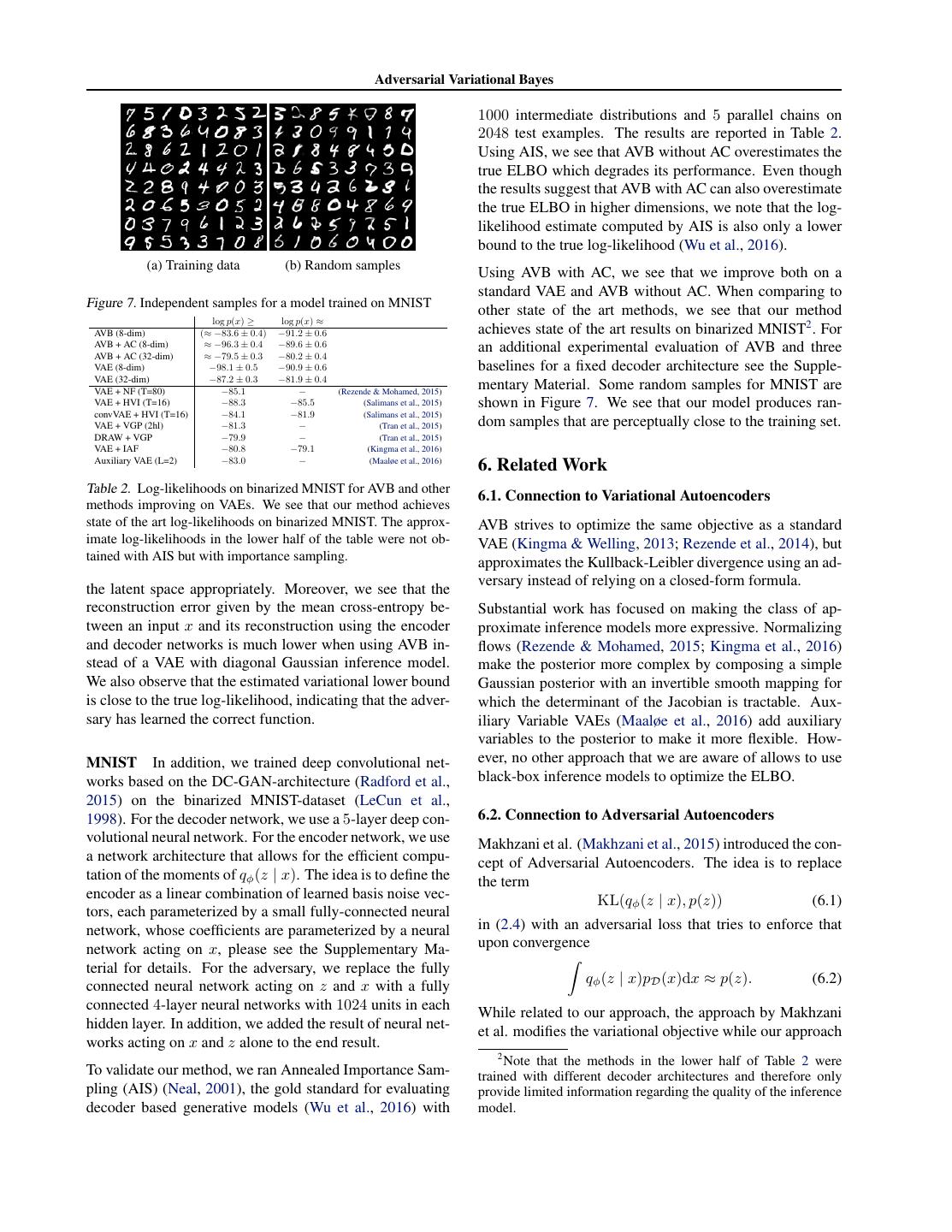
7 . Adversarial Variational Bayes 1000 intermediate distributions and 5 parallel chains on 2048 test examples. The results are reported in Table 2. Using AIS, we see that AVB without AC overestimates the true ELBO which degrades its performance. Even though the results suggest that AVB with AC can also overestimate the true ELBO in higher dimensions, we note that the log- likelihood estimate computed by AIS is also only a lower bound to the true log-likelihood (Wu et al., 2016). (a) Training data (b) Random samples Using AVB with AC, we see that we improve both on a standard VAE and AVB without AC. When comparing to Figure 7. Independent samples for a model trained on MNIST other state of the art methods, we see that our method log p(x) ≥ log p(x) ≈ AVB (8-dim) (≈ −83.6 ± 0.4) −91.2 ± 0.6 achieves state of the art results on binarized MNIST2 . For AVB + AC (8-dim) ≈ −96.3 ± 0.4 −89.6 ± 0.6 an additional experimental evaluation of AVB and three AVB + AC (32-dim) ≈ −79.5 ± 0.3 −80.2 ± 0.4 VAE (8-dim) −98.1 ± 0.5 −90.9 ± 0.6 baselines for a fixed decoder architecture see the Supple- VAE (32-dim) −87.2 ± 0.3 −81.9 ± 0.4 VAE + NF (T=80) −85.1 − (Rezende & Mohamed, 2015) mentary Material. Some random samples for MNIST are VAE + HVI (T=16) −88.3 −85.5 (Salimans et al., 2015) shown in Figure 7. We see that our model produces ran- convVAE + HVI (T=16) −84.1 −81.9 (Salimans et al., 2015) VAE + VGP (2hl) −81.3 − (Tran et al., 2015) dom samples that are perceptually close to the training set. DRAW + VGP −79.9 − (Tran et al., 2015) VAE + IAF −80.8 −79.1 (Kingma et al., 2016) Auxiliary VAE (L=2) −83.0 − (Maaløe et al., 2016) 6. Related Work Table 2. Log-likelihoods on binarized MNIST for AVB and other 6.1. Connection to Variational Autoencoders methods improving on VAEs. We see that our method achieves state of the art log-likelihoods on binarized MNIST. The approx- AVB strives to optimize the same objective as a standard imate log-likelihoods in the lower half of the table were not ob- VAE (Kingma & Welling, 2013; Rezende et al., 2014), but tained with AIS but with importance sampling. approximates the Kullback-Leibler divergence using an ad- the latent space appropriately. Moreover, we see that the versary instead of relying on a closed-form formula. reconstruction error given by the mean cross-entropy be- Substantial work has focused on making the class of ap- tween an input x and its reconstruction using the encoder proximate inference models more expressive. Normalizing and decoder networks is much lower when using AVB in- flows (Rezende & Mohamed, 2015; Kingma et al., 2016) stead of a VAE with diagonal Gaussian inference model. make the posterior more complex by composing a simple We also observe that the estimated variational lower bound Gaussian posterior with an invertible smooth mapping for is close to the true log-likelihood, indicating that the adver- which the determinant of the Jacobian is tractable. Aux- sary has learned the correct function. iliary Variable VAEs (Maaløe et al., 2016) add auxiliary variables to the posterior to make it more flexible. How- MNIST In addition, we trained deep convolutional net- ever, no other approach that we are aware of allows to use works based on the DC-GAN-architecture (Radford et al., black-box inference models to optimize the ELBO. 2015) on the binarized MNIST-dataset (LeCun et al., 1998). For the decoder network, we use a 5-layer deep con- 6.2. Connection to Adversarial Autoencoders volutional neural network. For the encoder network, we use Makhzani et al. (Makhzani et al., 2015) introduced the con- a network architecture that allows for the efficient compu- cept of Adversarial Autoencoders. The idea is to replace tation of the moments of qφ (z | x). The idea is to define the the term encoder as a linear combination of learned basis noise vec- KL(qφ (z | x), p(z)) (6.1) tors, each parameterized by a small fully-connected neural network, whose coefficients are parameterized by a neural in (2.4) with an adversarial loss that tries to enforce that network acting on x, please see the Supplementary Ma- upon convergence terial for details. For the adversary, we replace the fully qφ (z | x)pD (x)dx ≈ p(z). (6.2) connected neural network acting on z and x with a fully connected 4-layer neural networks with 1024 units in each While related to our approach, the approach by Makhzani hidden layer. In addition, we added the result of neural net- et al. modifies the variational objective while our approach works acting on x and z alone to the end result. 2 Note that the methods in the lower half of Table 2 were To validate our method, we ran Annealed Importance Sam- trained with different decoder architectures and therefore only pling (AIS) (Neal, 2001), the gold standard for evaluating provide limited information regarding the quality of the inference decoder based generative models (Wu et al., 2016) with model. 

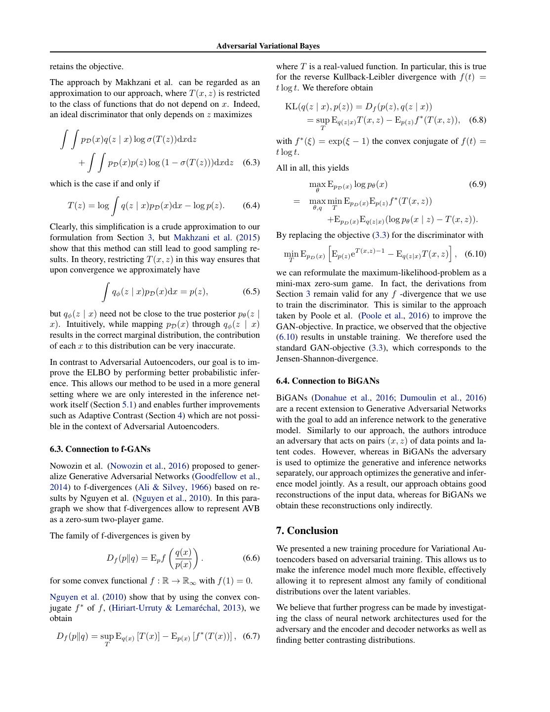
8 . Adversarial Variational Bayes retains the objective. where T is a real-valued function. In particular, this is true for the reverse Kullback-Leibler divergence with f (t) = The approach by Makhzani et al. can be regarded as an t log t. We therefore obtain approximation to our approach, where T (x, z) is restricted to the class of functions that do not depend on x. Indeed, KL(q(z | x), p(z)) = Df (p(z), q(z | x)) an ideal discriminator that only depends on z maximizes = sup Eq(z|x) T (x, z) − Ep(z) f ∗ (T (x, z)), (6.8) T pD (x)q(z | x) log σ(T (z))dxdz ∗ with f (ξ) = exp(ξ − 1) the convex conjugate of f (t) = t log t. + pD (x)p(z) log (1 − σ(T (z)))dxdz (6.3) All in all, this yields which is the case if and only if max EpD (x) log pθ (x) (6.9) θ = max min EpD (x) Ep(z) f ∗ (T (x, z)) T (z) = log q(z | x)pD (x)dx − log p(z). (6.4) θ,q T +EpD (x) Eq(z|x) (log pθ (x | z) − T (x, z)). Clearly, this simplification is a crude approximation to our formulation from Section 3, but Makhzani et al. (2015) By replacing the objective (3.3) for the discriminator with show that this method can still lead to good sampling re- min EpD (x) Ep(z) eT (x,z)−1 − Eq(z|x) T (x, z) , (6.10) sults. In theory, restricting T (x, z) in this way ensures that T upon convergence we approximately have we can reformulate the maximum-likelihood-problem as a mini-max zero-sum game. In fact, the derivations from qφ (z | x)pD (x)dx = p(z), (6.5) Section 3 remain valid for any f -divergence that we use to train the discriminator. This is similar to the approach but qφ (z | x) need not be close to the true posterior pθ (z | taken by Poole et al. (Poole et al., 2016) to improve the x). Intuitively, while mapping pD (x) through qφ (z | x) GAN-objective. In practice, we observed that the objective results in the correct marginal distribution, the contribution (6.10) results in unstable training. We therefore used the of each x to this distribution can be very inaccurate. standard GAN-objective (3.3), which corresponds to the In contrast to Adversarial Autoencoders, our goal is to im- Jensen-Shannon-divergence. prove the ELBO by performing better probabilistic infer- ence. This allows our method to be used in a more general 6.4. Connection to BiGANs setting where we are only interested in the inference net- BiGANs (Donahue et al., 2016; Dumoulin et al., 2016) work itself (Section 5.1) and enables further improvements are a recent extension to Generative Adversarial Networks such as Adaptive Contrast (Section 4) which are not possi- with the goal to add an inference network to the generative ble in the context of Adversarial Autoencoders. model. Similarly to our approach, the authors introduce an adversary that acts on pairs (x, z) of data points and la- 6.3. Connection to f-GANs tent codes. However, whereas in BiGANs the adversary Nowozin et al. (Nowozin et al., 2016) proposed to gener- is used to optimize the generative and inference networks alize Generative Adversarial Networks (Goodfellow et al., separately, our approach optimizes the generative and infer- 2014) to f-divergences (Ali & Silvey, 1966) based on re- ence model jointly. As a result, our approach obtains good sults by Nguyen et al. (Nguyen et al., 2010). In this para- reconstructions of the input data, whereas for BiGANs we graph we show that f-divergences allow to represent AVB obtain these reconstructions only indirectly. as a zero-sum two-player game. The family of f-divergences is given by 7. Conclusion q(x) We presented a new training procedure for Variational Au- Df (p q) = Ep f . (6.6) toencoders based on adversarial training. This allows us to p(x) make the inference model much more flexible, effectively for some convex functional f : R → R∞ with f (1) = 0. allowing it to represent almost any family of conditional distributions over the latent variables. Nguyen et al. (2010) show that by using the convex con- jugate f ∗ of f , (Hiriart-Urruty & Lemar´echal, 2013), we We believe that further progress can be made by investigat- obtain ing the class of neural network architectures used for the adversary and the encoder and decoder networks as well as Df (p q) = sup Eq(x) [T (x)] − Ep(x) [f ∗ (T (x))] , (6.7) finding better contrasting distributions. T 

9 . Adversarial Variational Bayes Acknowledgements Karaletsos, Theofanis. Adversarial message passing for graphical models. arXiv preprint arXiv:1612.05048, This work was supported by Microsoft Research through 2016. its PhD Scholarship Programme. Kingma, Diederik P and Welling, Max. Auto-encoding References variational bayes. arXiv preprint arXiv:1312.6114, 2013. Ali, Syed Mumtaz and Silvey, Samuel D. A general class of coefficients of divergence of one distribution from an- Kingma, Diederik P, Salimans, Tim, and Welling, Max. Im- other. Journal of the Royal Statistical Society. Series B proving variational inference with inverse autoregressive (Methodological), pp. 131–142, 1966. flow. arXiv preprint arXiv:1606.04934, 2016. Chen, Xi, Kingma, Diederik P, Salimans, Tim, Duan, Yan, Kucukelbir, Alp, Ranganath, Rajesh, Gelman, Andrew, and Dhariwal, Prafulla, Schulman, John, Sutskever, Ilya, and Blei, David. Automatic variational inference in stan. In Abbeel, Pieter. Variational lossy autoencoder. arXiv Advances in neural information processing systems, pp. preprint arXiv:1611.02731, 2016. 568–576, 2015. Dinh, Laurent, Sohl-Dickstein, Jascha, and Bengio, Samy. Larsen, Anders Boesen Lindbo, Sønderby, Søren Kaae, Density estimation using real nvp. arXiv preprint and Winther, Ole. Autoencoding beyond pixels arXiv:1605.08803, 2016. using a learned similarity metric. arXiv preprint arXiv:1512.09300, 2015. Donahue, Jeff, Kr¨ahenb¨uhl, Philipp, and Darrell, Trevor. Adversarial feature learning. arXiv preprint LeCun, Yann, Bottou, L´eon, Bengio, Yoshua, and Haffner, arXiv:1605.09782, 2016. Patrick. Gradient-based learning applied to document recognition. Proceedings of the IEEE, 86(11):2278– Dumoulin, Vincent, Belghazi, Ishmael, Poole, Ben, Lamb, 2324, 1998. Alex, Arjovsky, Martin, Mastropietro, Olivier, and Courville, Aaron. Adversarially learned inference. arXiv Li, Yingzhen and Liu, Qiang. Wild variational approxima- preprint arXiv:1606.00704, 2016. tions. In NIPS workshop on advances in approximate Bayesian inference, 2016. Friedman, Jerome, Hastie, Trevor, and Tibshirani, Robert. The elements of statistical learning, volume 1. Springer Liu, Qiang and Feng, Yihao. Two methods for wild vari- series in statistics Springer, Berlin, 2001. ational inference. arXiv preprint arXiv:1612.00081, 2016. Gelman, Andrew, Carlin, John B, Stern, Hal S, and Rubin, Donald B. Bayesian data analysis, volume 2. Chapman Liu, Ziwei, Luo, Ping, Wang, Xiaogang, and Tang, Xiaoou. & Hall/CRC Boca Raton, FL, USA, 2014. Deep learning face attributes in the wild. In Proceedings of International Conference on Computer Vision (ICCV), Goodfellow, Ian, Pouget-Abadie, Jean, Mirza, Mehdi, Xu, 2015. Bing, Warde-Farley, David, Ozair, Sherjil, Courville, Aaron, and Bengio, Yoshua. Generative adversarial nets. Maaløe, Lars, Sønderby, Casper Kaae, Sønderby, In Advances in Neural Information Processing Systems, Søren Kaae, and Winther, Ole. Auxiliary deep gener- pp. 2672–2680, 2014. ative models. arXiv preprint arXiv:1602.05473, 2016. He, Kaiming, Zhang, Xiangyu, Ren, Shaoqing, and Sun, Makhzani, Alireza, Shlens, Jonathon, Jaitly, Navdeep, and Jian. Deep residual learning for image recognition. arXiv Goodfellow, Ian. Adversarial autoencoders. arXiv preprint arXiv:1512.03385, 2015. preprint arXiv:1511.05644, 2015. Hiriart-Urruty, Jean-Baptiste and Lemar´echal, Claude. Neal, Radford M. Annealed importance sampling. Statis- Convex analysis and minimization algorithms I: funda- tics and Computing, 11(2):125–139, 2001. mentals, volume 305. Springer science & business me- dia, 2013. Nguyen, Anh, Yosinski, Jason, Bengio, Yoshua, Dosovit- skiy, Alexey, and Clune, Jeff. Plug & play generative Hornik, Kurt, Stinchcombe, Maxwell, and White, Halbert. networks: Conditional iterative generation of images in Multilayer feedforward networks are universal approxi- latent space. arXiv preprint arXiv:1612.00005, 2016. mators. Neural networks, 2(5):359–366, 1989. Nguyen, XuanLong, Wainwright, Martin J, and Jordan, Husz´ar, Ferenc. Variational inference using implicit distri- Michael I. Estimating divergence functionals and the butions. arXiv preprint arXiv:1702.08235, 2017. likelihood ratio by convex risk minimization. IEEE 

10 . Adversarial Variational Bayes Transactions on Information Theory, 56(11):5847–5861, Wu, Yuhuai, Burda, Yuri, Salakhutdinov, Ruslan, and 2010. Grosse, Roger. On the quantitative analysis of decoder-based generative models. arXiv preprint Nowozin, Sebastian, Cseke, Botond, and Tomioka, Ry- arXiv:1611.04273, 2016. ota. f-gan: Training generative neural samplers us- ing variational divergence minimization. arXiv preprint arXiv:1606.00709, 2016. Poole, Ben, Alemi, Alexander A, Sohl-Dickstein, Jascha, and Angelova, Anelia. Improved generator objectives for gans. arXiv preprint arXiv:1612.02780, 2016. Radford, Alec, Metz, Luke, and Chintala, Soumith. Un- supervised representation learning with deep convolu- tional generative adversarial networks. arXiv preprint arXiv:1511.06434, 2015. Ranganath, Rajesh, Tran, Dustin, Altosaar, Jaan, and Blei, David. Operator variational inference. In Advances in Neural Information Processing Systems, pp. 496–504, 2016. Rezende, Danilo Jimenez and Mohamed, Shakir. Varia- tional inference with normalizing flows. arXiv preprint arXiv:1505.05770, 2015. Rezende, Danilo Jimenez, Mohamed, Shakir, and Wier- stra, Daan. Stochastic backpropagation and approxi- mate inference in deep generative models. arXiv preprint arXiv:1401.4082, 2014. Salimans, Tim, Kingma, Diederik P, Welling, Max, et al. Markov chain monte carlo and variational inference: Bridging the gap. In ICML, volume 37, pp. 1218–1226, 2015. Stan Development Team. Stan modeling language users guide and reference manual, Version 2.14.0, 2016. URL http://mc-stan.org. Szabo, Zolt´an. Information theoretical estimators (ite) tool- box. 2013. Tran, Dustin, Ranganath, Rajesh, and Blei, David M. The variational gaussian process. arXiv preprint arXiv:1511.06499, 2015. van den Oord, Aaron, Kalchbrenner, Nal, Espeholt, Lasse, Vinyals, Oriol, Graves, Alex, et al. Conditional im- age generation with pixelcnn decoders. In Advances In Neural Information Processing Systems, pp. 4790–4798, 2016a. van den Oord, Aaron van den, Kalchbrenner, Nal, and Kavukcuoglu, Koray. Pixel recurrent neural networks. arXiv preprint arXiv:1601.06759, 2016b. 

11 . Supplementary Material for Adversarial Variational Bayes: Unifying Variational Autoencoders and Generative Adversarial Networks Lars Mescheder 1 Sebastian Nowozin 2 Andreas Geiger 1 3 Abstract To apply our method in practice, we need to obtain unbi- In the main text we derived Adversarial Varia- ased gradients of the ELBO. As it turns out, this can be tional Bayes (AVB) and demonstrated its useful- achieved by taking the gradients w.r.t. a fixed optimal dis- ness both for black-box Variational Inference and criminator. This is a consequence of the following Propo- for learning latent variable models. This doc- sition: ument contains proofs that were omitted in the Proposition 2. We have main text as well as some further details about Eqφ (z|x) (∇φ T ∗ (x, z)) = 0. (3.6) the experiments and additional results. Proof. By Proposition 1, I. Proofs Eqφ (z|x) (∇φ T ∗ (x, z)) This section contains the proofs that were omitted in the = Eqφ (z|x) (∇φ log qφ (z | x)) . (I.5) main text. For an arbitrary family of probability densities qφ we have The derivation of AVB in Section 3.1 relies on the fact that we have an explicit representation of the optimal discrim- ∇φ qφ (z) inator T ∗ (x, z). This was stated in the following Proposi- Eqφ (∇φ log qφ ) = qφ (z) dz qφ (z) tion: Proposition 1. For pθ (x | z) and qφ (z | x) fixed, the opti- = ∇φ qφ (z)dz = ∇φ 1 = 0. (I.6) mal discriminator T ∗ according to the objective in (3.3) is given by Together with (I.5), this implies (3.6). T ∗ (x, z) = log qφ (z | x) − log p(z). (3.4) In Section 3.3 we characterized the Nash-equilibria of the two-player game defined by our algorithm. The follow- Proof. As in the proof of Proposition 1 in Goodfellow et al. ing Proposition shows that in the nonparametric limit for (2014), we rewrite the objective in (3.3) as T (x, z) any Nash-equilibrium defines a global optimum of the variational lower bound: pD (x)qφ (z | x) log σ(T (x, z)) Proposition 3. Assume that T can represent any function of two variables. If (θ∗ , φ∗ , T ∗ ) defines a Nash-equilibrium + pD (x)p(z) log(1 − σ(T (x, z)) dxdz. (I.1) of the two-player game defined by (3.3) and (3.7), This integral is maximal as a function of T (x, z) if and only then if the integrand is maximal for every (x, z). However, the T ∗ (x, z) = log qφ∗ (z | x) − log p(z) (3.8) function ∗ ∗ t → a log(t) + b log(1 − t) (I.2) and (θ , φ ) is a global optimum of the variational lower a bound in (2.4). attains its maximum at t = a+b , showing that qφ (z | x) Proof. If (θ∗ , φ∗ , T ∗ ) defines a Nash-equilibrium, Propo- σ(T ∗ (x, z)) = (I.3) qφ (z | x) + p(z) sition 1 shows (3.8). Inserting (3.8) into (3.5) shows that (φ∗ , θ∗ ) maximizes or, equivalently, T ∗ (x, z) = log qφ (z | x) − log p(z). (I.4) EpD (x) Eqφ (z|x) − log qφ∗ (z | x) + log p(z) + log pθ (x | z) (I.7) 

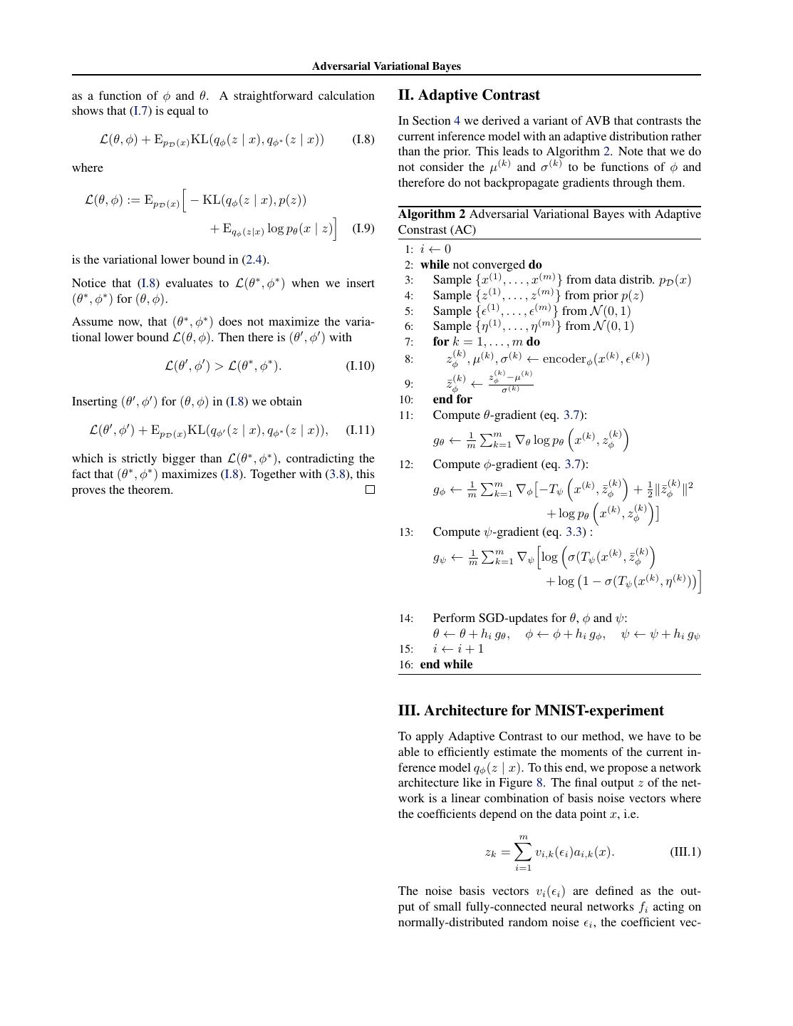
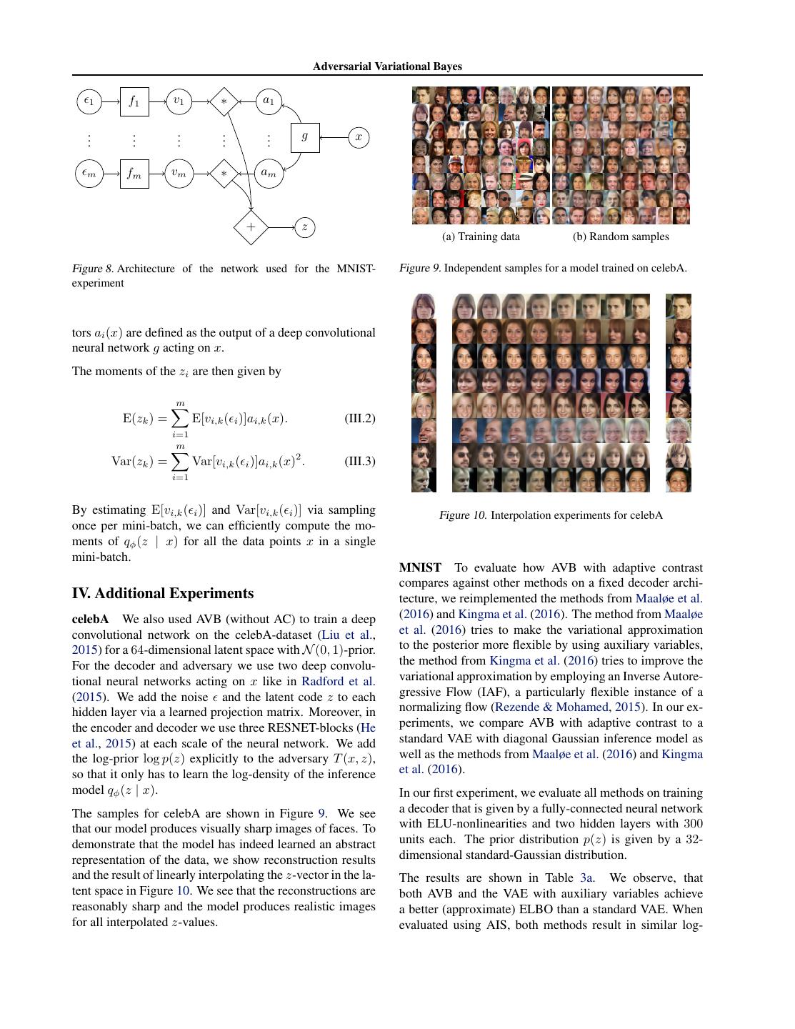
12 . Adversarial Variational Bayes as a function of φ and θ. A straightforward calculation II. Adaptive Contrast shows that (I.7) is equal to In Section 4 we derived a variant of AVB that contrasts the L(θ, φ) + EpD (x) KL(qφ (z | x), qφ∗ (z | x)) (I.8) current inference model with an adaptive distribution rather than the prior. This leads to Algorithm 2. Note that we do where not consider the µ(k) and σ (k) to be functions of φ and therefore do not backpropagate gradients through them. L(θ, φ) := EpD (x) − KL(qφ (z | x), p(z)) Algorithm 2 Adversarial Variational Bayes with Adaptive + Eqφ (z|x) log pθ (x | z) (I.9) Constrast (AC) 1: i ← 0 is the variational lower bound in (2.4). 2: while not converged do Notice that (I.8) evaluates to L(θ∗ , φ∗ ) when we insert 3: Sample {x(1) , . . . , x(m) } from data distrib. pD (x) (θ∗ , φ∗ ) for (θ, φ). 4: Sample {z (1) , . . . , z (m) } from prior p(z) 5: Sample { (1) , . . . , (m) } from N (0, 1) Assume now, that (θ∗ , φ∗ ) does not maximize the varia- 6: Sample {η (1) , . . . , η (m) } from N (0, 1) tional lower bound L(θ, φ). Then there is (θ , φ ) with 7: for k = 1, . . . , m do (k) 8: zφ , µ(k) , σ (k) ← encoderφ (x(k) , (k) ) L(θ , φ ) > L(θ∗ , φ∗ ). (I.10) (k) (k) z −µ(k) 9: z¯φ ← φ σ(k) Inserting (θ , φ ) for (θ, φ) in (I.8) we obtain 10: end for 11: Compute θ-gradient (eq. 3.7): L(θ , φ ) + EpD (x) KL(qφ (z | x), qφ∗ (z | x)), (I.11) 1 m (k) gθ ← m k=1 ∇θ log pθ x(k) , zφ which is strictly bigger than L(θ∗ , φ∗ ), contradicting the 12: Compute φ-gradient (eq. 3.7): fact that (θ∗ , φ∗ ) maximizes (I.8). Together with (3.8), this 1 m (k) 1 (k) 2 proves the theorem. gφ ← m k=1 ∇φ −Tψ x(k) , z¯φ + 2 z¯φ (k) + log pθ x(k) , zφ 13: Compute ψ-gradient (eq. 3.3) : 1 m (k) gψ ← m k=1 ∇ψ log σ(Tψ (x(k) , z¯φ + log 1 − σ(Tψ (x(k) , η (k) ) 14: Perform SGD-updates for θ, φ and ψ: θ ← θ + hi gθ , φ ← φ + hi gφ , ψ ← ψ + hi gψ 15: i←i+1 16: end while III. Architecture for MNIST-experiment To apply Adaptive Contrast to our method, we have to be able to efficiently estimate the moments of the current in- ference model qφ (z | x). To this end, we propose a network architecture like in Figure 8. The final output z of the net- work is a linear combination of basis noise vectors where the coefficients depend on the data point x, i.e. m zk = vi,k ( i )ai,k (x). (III.1) i=1 The noise basis vectors vi ( i ) are defined as the out- put of small fully-connected neural networks fi acting on normally-distributed random noise i , the coefficient vec- 

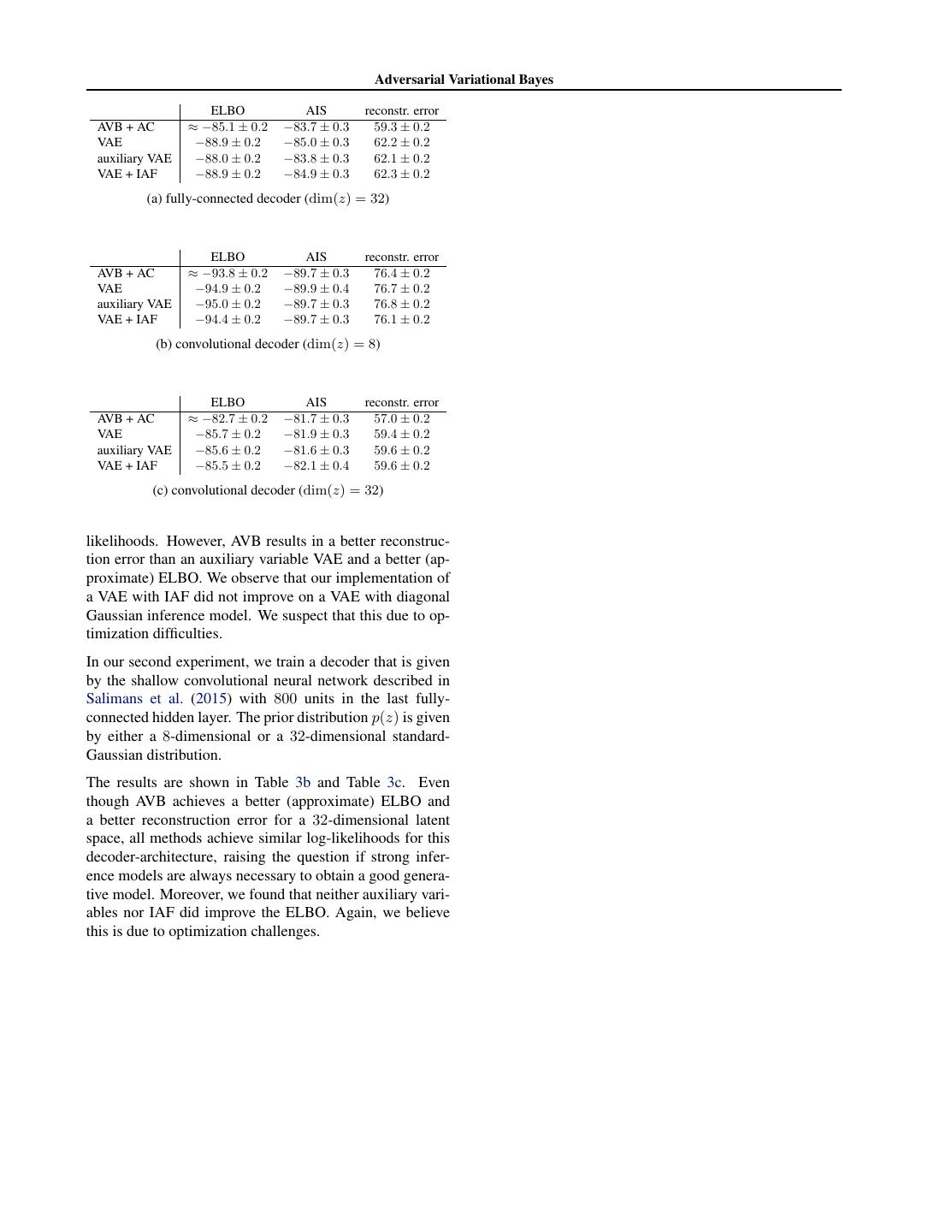
13 . Adversarial Variational Bayes 1 f1 v1 ∗ a1 .. .. .. .. .. g x . . . . . m fm vm ∗ am + z (a) Training data (b) Random samples Figure 8. Architecture of the network used for the MNIST- Figure 9. Independent samples for a model trained on celebA. experiment tors ai (x) are defined as the output of a deep convolutional neural network g acting on x. The moments of the zi are then given by m E(zk ) = E[vi,k ( i )]ai,k (x). (III.2) i=1 m Var(zk ) = Var[vi,k ( i )]ai,k (x)2 . (III.3) i=1 By estimating E[vi,k ( i )] and Var[vi,k ( i )] via sampling Figure 10. Interpolation experiments for celebA once per mini-batch, we can efficiently compute the mo- ments of qφ (z | x) for all the data points x in a single mini-batch. MNIST To evaluate how AVB with adaptive contrast compares against other methods on a fixed decoder archi- IV. Additional Experiments tecture, we reimplemented the methods from Maaløe et al. celebA We also used AVB (without AC) to train a deep (2016) and Kingma et al. (2016). The method from Maaløe convolutional network on the celebA-dataset (Liu et al., et al. (2016) tries to make the variational approximation 2015) for a 64-dimensional latent space with N (0, 1)-prior. to the posterior more flexible by using auxiliary variables, For the decoder and adversary we use two deep convolu- the method from Kingma et al. (2016) tries to improve the tional neural networks acting on x like in Radford et al. variational approximation by employing an Inverse Autore- (2015). We add the noise and the latent code z to each gressive Flow (IAF), a particularly flexible instance of a hidden layer via a learned projection matrix. Moreover, in normalizing flow (Rezende & Mohamed, 2015). In our ex- the encoder and decoder we use three RESNET-blocks (He periments, we compare AVB with adaptive contrast to a et al., 2015) at each scale of the neural network. We add standard VAE with diagonal Gaussian inference model as the log-prior log p(z) explicitly to the adversary T (x, z), well as the methods from Maaløe et al. (2016) and Kingma so that it only has to learn the log-density of the inference et al. (2016). model qφ (z | x). In our first experiment, we evaluate all methods on training The samples for celebA are shown in Figure 9. We see a decoder that is given by a fully-connected neural network that our model produces visually sharp images of faces. To with ELU-nonlinearities and two hidden layers with 300 demonstrate that the model has indeed learned an abstract units each. The prior distribution p(z) is given by a 32- representation of the data, we show reconstruction results dimensional standard-Gaussian distribution. and the result of linearly interpolating the z-vector in the la- The results are shown in Table 3a. We observe, that tent space in Figure 10. We see that the reconstructions are both AVB and the VAE with auxiliary variables achieve reasonably sharp and the model produces realistic images a better (approximate) ELBO than a standard VAE. When for all interpolated z-values. evaluated using AIS, both methods result in similar log- 

14 . Adversarial Variational Bayes ELBO AIS reconstr. error AVB + AC ≈ −85.1 ± 0.2 −83.7 ± 0.3 59.3 ± 0.2 VAE −88.9 ± 0.2 −85.0 ± 0.3 62.2 ± 0.2 auxiliary VAE −88.0 ± 0.2 −83.8 ± 0.3 62.1 ± 0.2 VAE + IAF −88.9 ± 0.2 −84.9 ± 0.3 62.3 ± 0.2 (a) fully-connected decoder (dim(z) = 32) ELBO AIS reconstr. error AVB + AC ≈ −93.8 ± 0.2 −89.7 ± 0.3 76.4 ± 0.2 VAE −94.9 ± 0.2 −89.9 ± 0.4 76.7 ± 0.2 auxiliary VAE −95.0 ± 0.2 −89.7 ± 0.3 76.8 ± 0.2 VAE + IAF −94.4 ± 0.2 −89.7 ± 0.3 76.1 ± 0.2 (b) convolutional decoder (dim(z) = 8) ELBO AIS reconstr. error AVB + AC ≈ −82.7 ± 0.2 −81.7 ± 0.3 57.0 ± 0.2 VAE −85.7 ± 0.2 −81.9 ± 0.3 59.4 ± 0.2 auxiliary VAE −85.6 ± 0.2 −81.6 ± 0.3 59.6 ± 0.2 VAE + IAF −85.5 ± 0.2 −82.1 ± 0.4 59.6 ± 0.2 (c) convolutional decoder (dim(z) = 32) likelihoods. However, AVB results in a better reconstruc- tion error than an auxiliary variable VAE and a better (ap- proximate) ELBO. We observe that our implementation of a VAE with IAF did not improve on a VAE with diagonal Gaussian inference model. We suspect that this due to op- timization difficulties. In our second experiment, we train a decoder that is given by the shallow convolutional neural network described in Salimans et al. (2015) with 800 units in the last fully- connected hidden layer. The prior distribution p(z) is given by either a 8-dimensional or a 32-dimensional standard- Gaussian distribution. The results are shown in Table 3b and Table 3c. Even though AVB achieves a better (approximate) ELBO and a better reconstruction error for a 32-dimensional latent space, all methods achieve similar log-likelihoods for this decoder-architecture, raising the question if strong infer- ence models are always necessary to obtain a good genera- tive model. Moreover, we found that neither auxiliary vari- ables nor IAF did improve the ELBO. Again, we believe this is due to optimization challenges.