Regression

1 .Regression Hung-yi Lee 李宏毅 

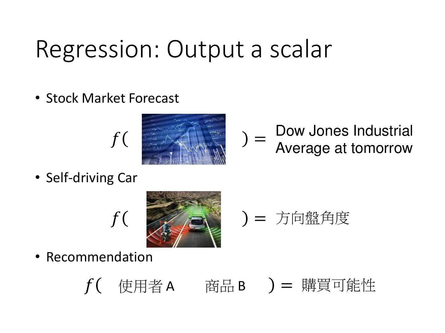
2 .Regression: Output a scalar • Stock Market Forecast 𝑓 = Dow Jones Industrial Average at tomorrow • Self-driving Car 𝑓 = 方向盤角度 • Recommendation 𝑓 使用者 A 商品 B = 購買可能性 

3 .Example Application • Estimating the Combat Power (CP) of a pokemon after evolution 𝑥𝑐𝑝 CP after 𝑓 = evolution 𝑦 𝑥𝑠 𝑥 𝑥ℎ𝑝 𝑥𝑤 𝑥ℎ 

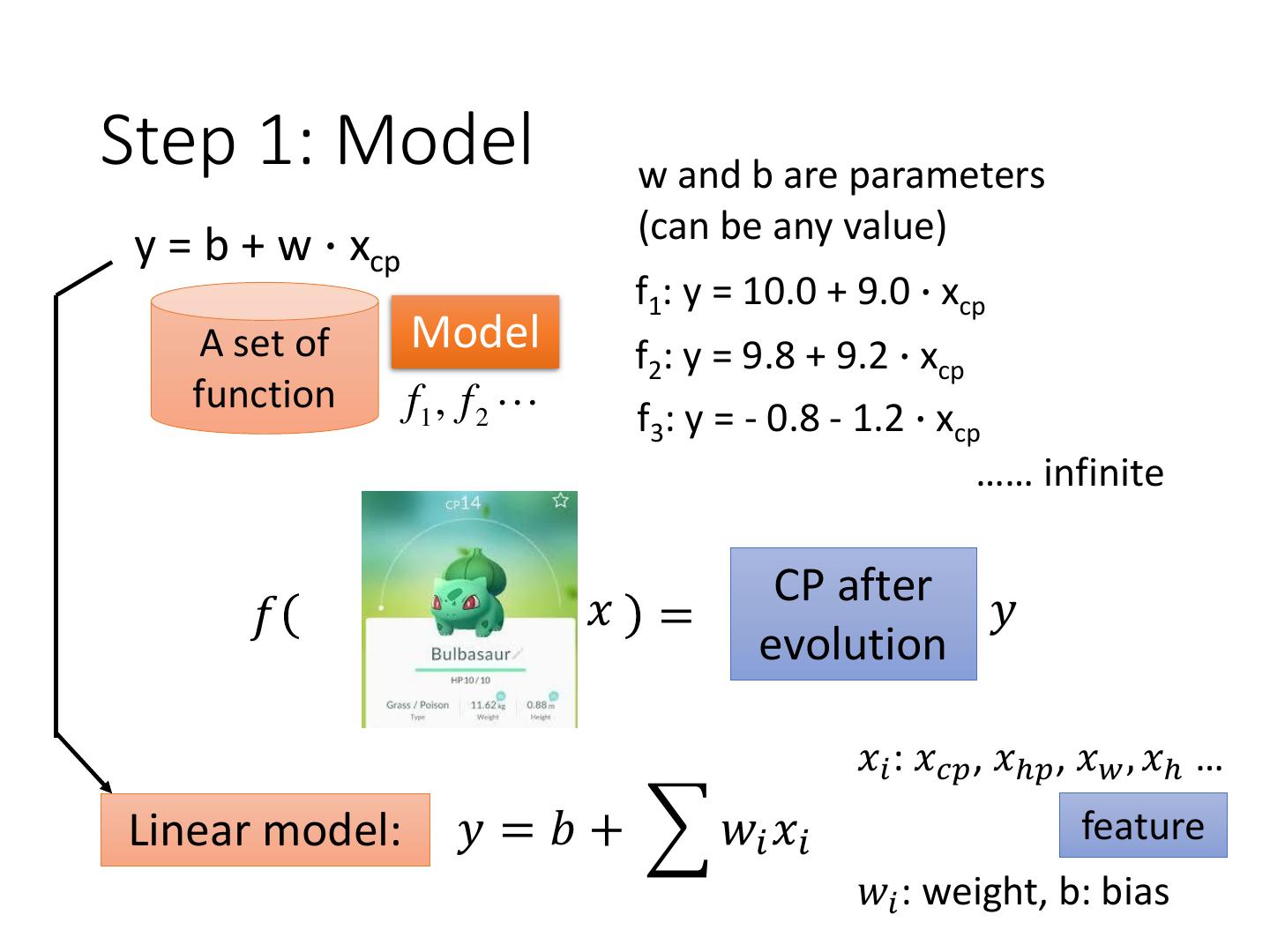
4 .Step 1: Model w and b are parameters y = b + w ∙ xcp (can be any value) f1: y = 10.0 + 9.0 ∙ xcp A set of Model f2: y = 9.8 + 9.2 ∙ xcp function f1 , f 2  f3: y = - 0.8 - 1.2 ∙ xcp …… infinite CP after 𝑓 𝑥 = 𝑦 evolution 𝑥𝑖 : 𝑥𝑐𝑝 , 𝑥ℎ𝑝 , 𝑥𝑤 , 𝑥ℎ … Linear model: 𝑦 = 𝑏 + ෍ 𝑤𝑖 𝑥𝑖 feature 𝑤𝑖 : weight, b: bias 

5 .Step 2: Goodness of Function y = b + w ∙ xcp function function A set of Model input: Output (scalar): function f1 , f 2  𝑦ො 1 𝑥1 𝑦ො 2 𝑥2 Training Data 

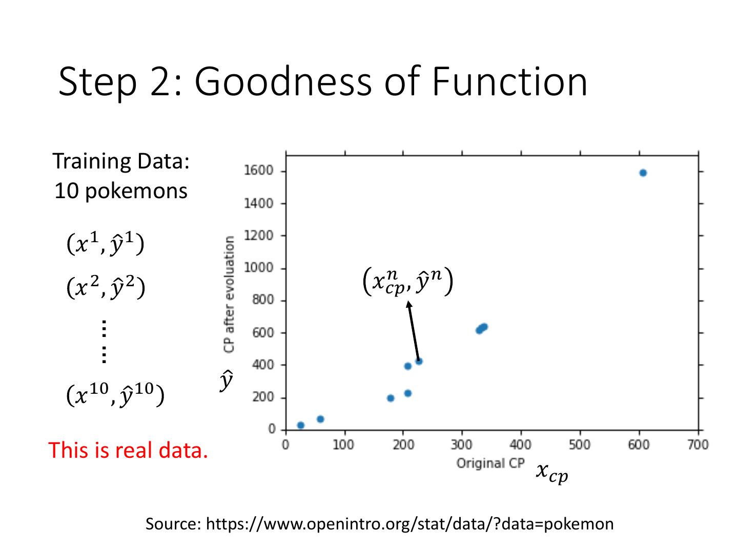
6 . Step 2: Goodness of Function Training Data: 10 pokemons 𝑥 1 , 𝑦ො 1 𝑛 ,𝑦 𝑥𝑐𝑝 ො𝑛 𝑥 2 , 𝑦ො 2 …… 𝑦ො 𝑥 10 , 𝑦ො 10 This is real data. 𝑥𝑐𝑝 Source: https://www.openintro.org/stat/data/?data=pokemon 

7 .Step 2: Goodness of Function y = b + w ∙ xcp Loss function 𝐿: A set of Model Input: a function, output: function f1 , f 2  how bad it is 10 Estimation error 2 Goodness of L 𝑓 =෍ 𝑦ො 𝑛 −𝑓 𝑛 𝑥𝑐𝑝 function f 𝑛=1 Sum over examples Estimated y based on input function Training L 𝑤, 𝑏 10 2 Data = ෍ 𝑦ො 𝑛 − 𝑏 + 𝑤 ∙ 𝑥𝑐𝑝 𝑛 𝑛=1 

8 .Step 2: Goodness of Function 10 2 L 𝑤, 𝑏 = ෍ 𝑦ො 𝑛 − 𝑏+𝑤∙ 𝑛 𝑥𝑐𝑝 • Loss Function 𝑛=1 Each point in smallest the figure is a function y = - 180 - 2 ∙ xcp The color represents L 𝑤, 𝑏 . Very large (true example) 

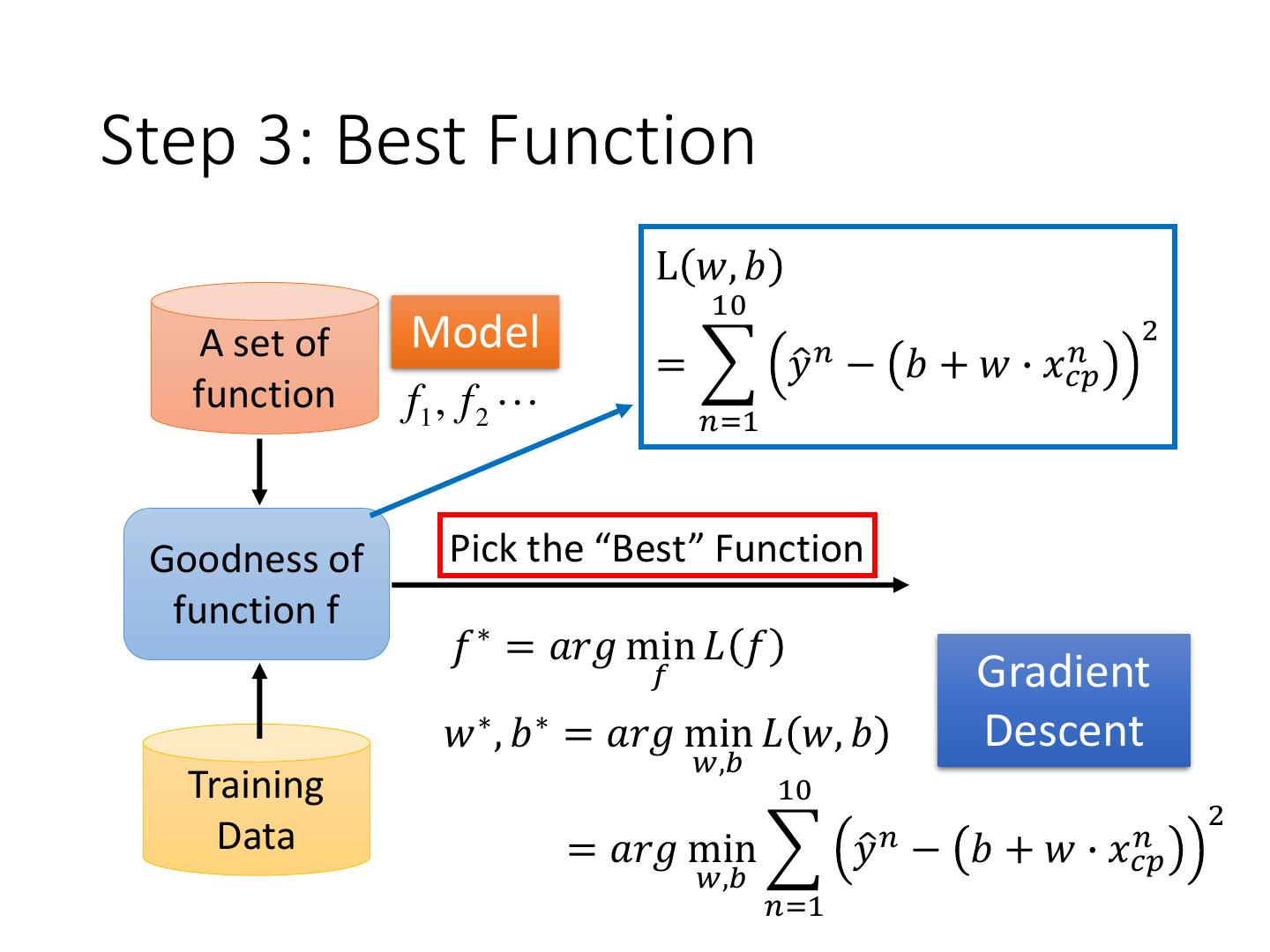
9 .Step 3: Best Function L 𝑤, 𝑏 10 A set of Model 2 =෍ 𝑦ො 𝑛 − 𝑏+𝑤∙ 𝑛 𝑥𝑐𝑝 function f1 , f 2  𝑛=1 Goodness of Pick the “Best” Function function f 𝑓 ∗ = 𝑎𝑟𝑔 min 𝐿 𝑓 𝑓 Gradient 𝑤 ∗ , 𝑏 ∗ = 𝑎𝑟𝑔 min 𝐿 𝑤, 𝑏 Descent 𝑤,𝑏 Training 10 2 Data = 𝑎𝑟𝑔 min ෍ 𝑦ො 𝑛 − 𝑏+𝑤∙ 𝑛 𝑥𝑐𝑝 𝑤,𝑏 𝑛=1 

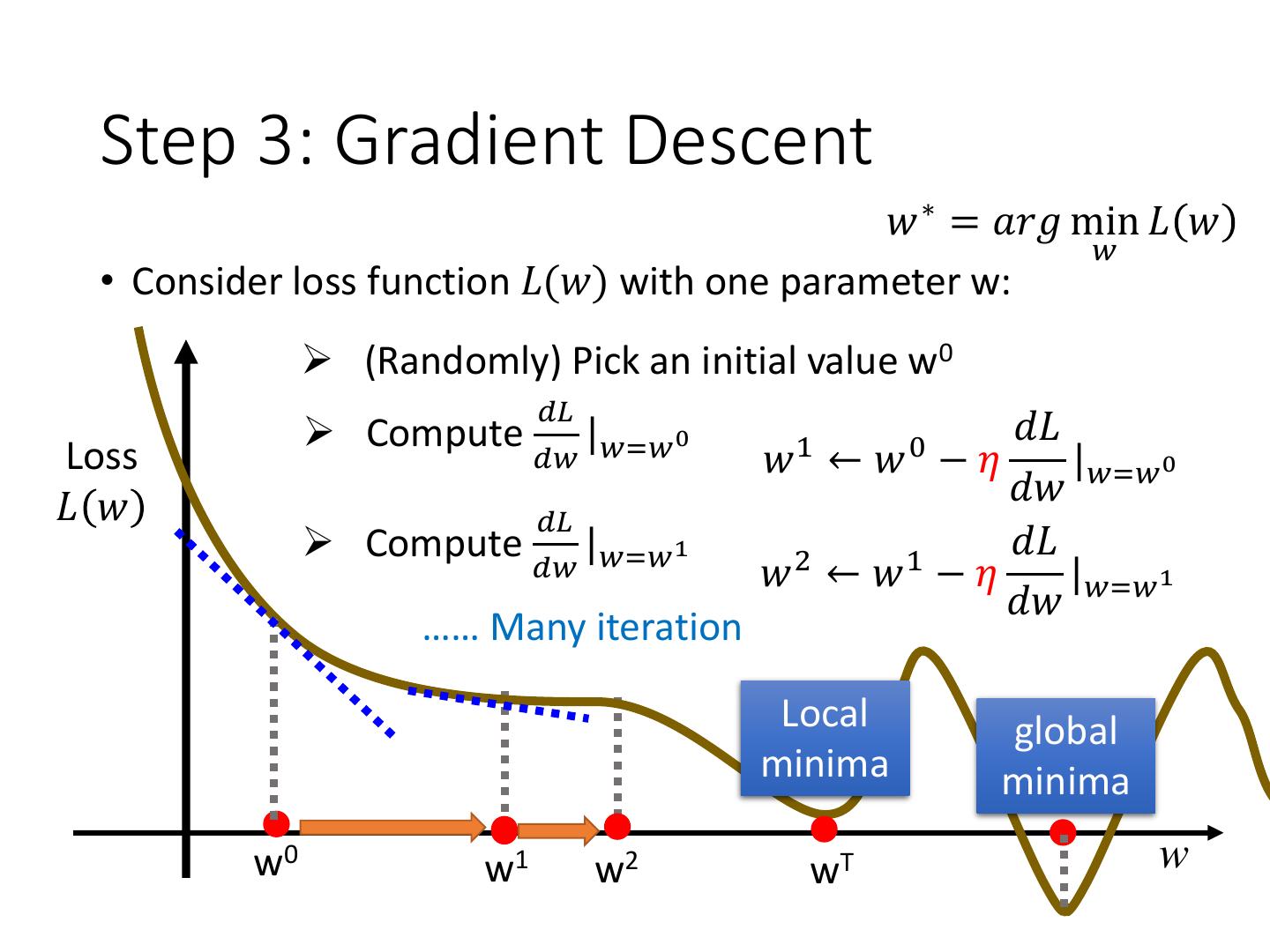
10 . http://chico386.pixnet.net/al bum/photo/171572850 Step 3: Gradient Descent 𝑤 ∗ = 𝑎𝑟𝑔 min 𝐿 𝑤 𝑤 • Consider loss function 𝐿(𝑤) with one parameter w:  (Randomly) Pick an initial value w0 𝑑𝐿  Compute | 0 Loss 𝑑𝑤 𝑤=𝑤 𝐿 𝑤 Negative Increase w Positive Decrease w w0 w 

11 . http://chico386.pixnet.net/al bum/photo/171572850 Step 3: Gradient Descent 𝑤 ∗ = 𝑎𝑟𝑔 min 𝐿 𝑤 𝑤 • Consider loss function 𝐿(𝑤) with one parameter w:  (Randomly) Pick an initial value w0 𝑑𝐿  Compute | 0 𝑑𝐿 Loss 𝑑𝑤 𝑤=𝑤 𝑤1 ← 𝑤0 −𝜂 |𝑤=𝑤 0 𝐿 𝑤 𝑑𝑤 η is called w0 𝑑𝐿 “learning rate” w −𝜂 |𝑤=𝑤 0 𝑑𝑤 

12 . Step 3: Gradient Descent 𝑤 ∗ = 𝑎𝑟𝑔 min 𝐿 𝑤 𝑤 • Consider loss function 𝐿(𝑤) with one parameter w:  (Randomly) Pick an initial value w0 𝑑𝐿  Compute | 0 1 𝑑𝐿 0 Loss 𝑑𝑤 𝑤=𝑤 𝑤 ←𝑤 −𝜂 |𝑤=𝑤 0 𝐿 𝑤 𝑑𝑤 𝑑𝐿  Compute | 1 𝑑𝐿 𝑑𝑤 𝑤=𝑤 2 1 𝑤 ←𝑤 −𝜂 |𝑤=𝑤 1 𝑑𝑤 …… Many iteration Local global minima minima w0 w1 w2 wT w 

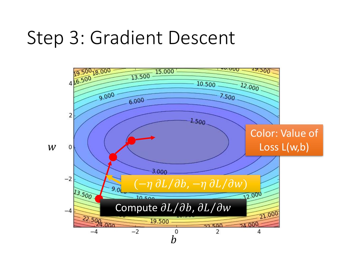
13 . 𝜕𝐿 𝛻𝐿 = 𝜕𝑤 Step 3: Gradient Descent 𝜕𝐿 𝜕𝑏 gradient • How about two parameters? 𝑤 ∗ , 𝑏 ∗ = 𝑎𝑟𝑔 min 𝐿 𝑤, 𝑏 𝑤,𝑏  (Randomly) Pick an initial value w0, b0 𝜕𝐿 𝜕𝐿  Compute |𝑤=𝑤 0 ,𝑏=𝑏0 , |𝑤=𝑤 0 ,𝑏=𝑏0 𝜕𝑤 𝜕𝑏 𝜕𝐿 𝜕𝐿 𝑤1 ← 𝑤0 −𝜂 |𝑤=𝑤 0 ,𝑏=𝑏0 𝑏1 ← 𝑏0 − 𝜂 |𝑤=𝑤 0 ,𝑏=𝑏0 𝜕𝑤 𝜕𝑏 𝜕𝐿 𝜕𝐿  Compute |𝑤=𝑤 1 ,𝑏=𝑏1 , |𝑤=𝑤 1 ,𝑏=𝑏1 𝜕𝑤 𝜕𝑏 2 𝜕𝐿 1 𝜕𝐿 𝑤 ←𝑤 −𝜂 |𝑤=𝑤 1 ,𝑏=𝑏1 𝑏2 ← 𝑏1 − 𝜂 |𝑤=𝑤 1 ,𝑏=𝑏1 𝜕𝑤 𝜕𝑏 

14 .Step 3: Gradient Descent Color: Value of 𝑤 Loss L(w,b) (−𝜂 𝜕𝐿Τ𝜕𝑏, −𝜂 𝜕𝐿Τ𝜕𝑤) Compute 𝜕𝐿Τ𝜕𝑏, 𝜕𝐿Τ𝜕𝑤 𝑏 

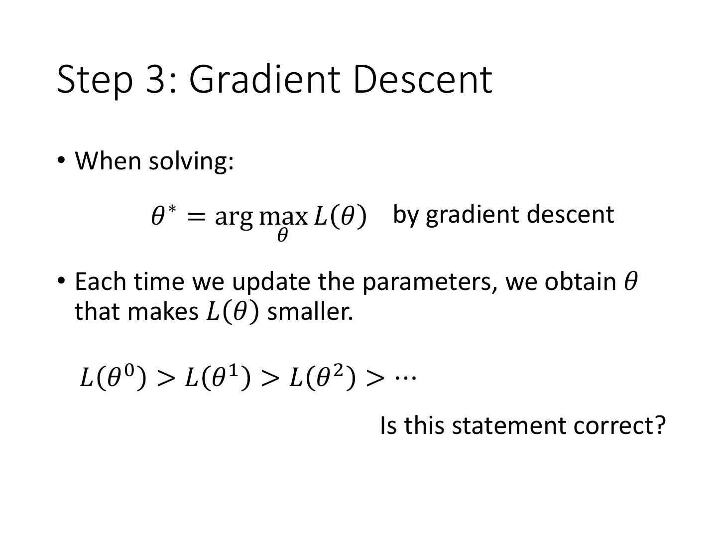
15 .Step 3: Gradient Descent • When solving: 𝜃 ∗ = arg max 𝐿 𝜃 by gradient descent 𝜃 • Each time we update the parameters, we obtain 𝜃 that makes 𝐿 𝜃 smaller. 𝐿 𝜃 0 > 𝐿 𝜃1 > 𝐿 𝜃 2 > ⋯ Is this statement correct? 

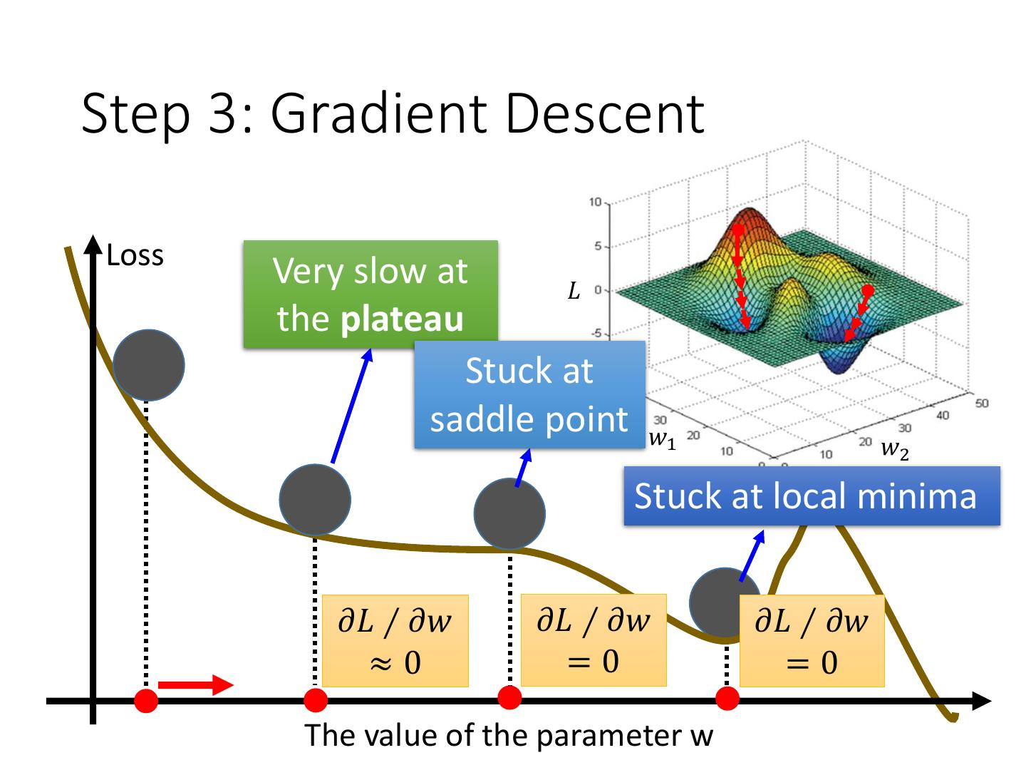
16 .Step 3: Gradient Descent Loss Very slow at 𝐿 the plateau Stuck at saddle point 𝑤1 𝑤2 Stuck at local minima 𝜕𝐿 ∕ 𝜕𝑤 𝜕𝐿 ∕ 𝜕𝑤 𝜕𝐿 ∕ 𝜕𝑤 ≈0 =0 =0 The value of the parameter w 

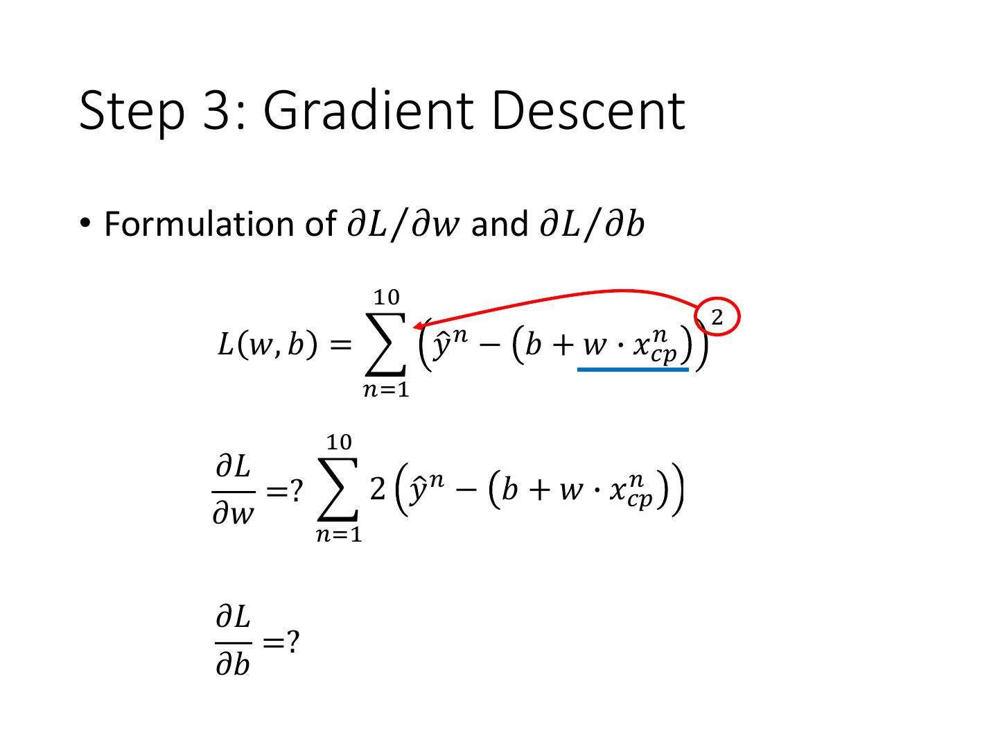
17 .Step 3: Gradient Descent • Formulation of 𝜕𝐿Τ𝜕𝑤 and 𝜕𝐿Τ𝜕𝑏 10 2 𝑛 𝑛 𝐿 𝑤, 𝑏 = ෍ 𝑦ො − 𝑏 + 𝑤 ∙ 𝑥𝑐𝑝 𝑛=1 10 𝜕𝐿 =? ෍ 2 𝑦ො 𝑛 − 𝑏 + 𝑤 ∙ 𝑥𝑐𝑝 𝑛 𝑛 −𝑥𝑐𝑝 𝜕𝑤 𝑛=1 𝜕𝐿 =? 𝜕𝑏 

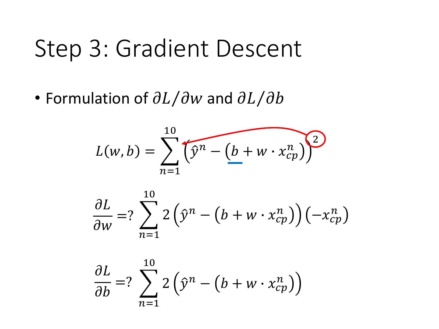
18 .Step 3: Gradient Descent • Formulation of 𝜕𝐿Τ𝜕𝑤 and 𝜕𝐿Τ𝜕𝑏 10 2 𝑛 𝑛 𝐿 𝑤, 𝑏 = ෍ 𝑦ො − 𝑏 + 𝑤 ∙ 𝑥𝑐𝑝 𝑛=1 10 𝜕𝐿 =? ෍ 2 𝑦ො 𝑛 − 𝑏 + 𝑤 ∙ 𝑥𝑐𝑝 𝑛 𝑛 −𝑥𝑐𝑝 𝜕𝑤 𝑛=1 10 𝜕𝐿 =? ෍ 2 𝑦ො 𝑛 − 𝑏 + 𝑤 ∙ 𝑥𝑐𝑝 𝑛 −1 𝜕𝑏 𝑛=1 

19 .Step 3: Gradient Descent 

20 . How’s the results? Training Data y = b + w ∙ xcp 𝑒1 b = -188.4 w = 2.7 Average Error on Training Data 𝑒2 10 1 = ෍ 𝑒 𝑛 = 31.9 10 𝑛=1 

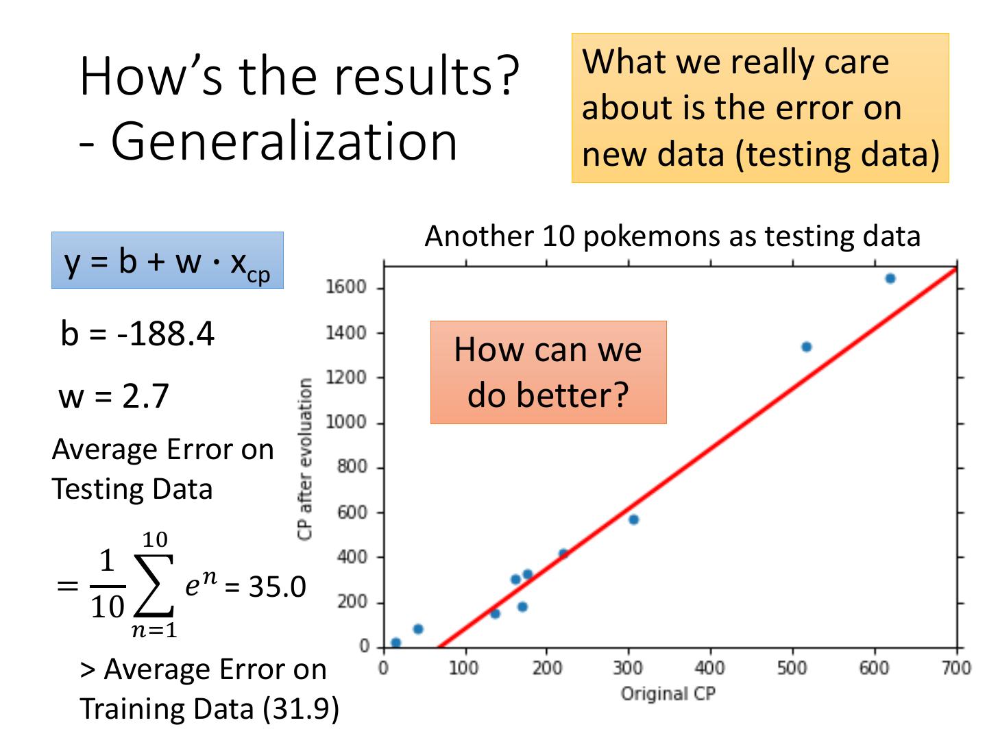
21 . What we really care How’s the results? about is the error on - Generalization new data (testing data) Another 10 pokemons as testing data y = b + w ∙ xcp b = -188.4 How can we w = 2.7 do better? Average Error on Testing Data 10 1 = ෍ 𝑒 𝑛 = 35.0 10 𝑛=1 > Average Error on Training Data (31.9) 

22 .Selecting another Model y = b + w1 ∙ xcp + w2 ∙ (xcp)2 Best Function b = -10.3 w1 = 1.0, w2 = 2.7 x 10-3 Average Error = 15.4 Testing: Average Error = 18.4 Better! Could it be even better? 

23 .Selecting another Model y = b + w1 ∙ xcp + w2 ∙ (xcp)2 + w3 ∙ (xcp)3 Best Function b = 6.4, w1 = 0.66 w2 = 4.3 x 10-3 w3 = -1.8 x 10-6 Average Error = 15.3 Testing: Average Error = 18.1 Slightly better. How about more complex model? 

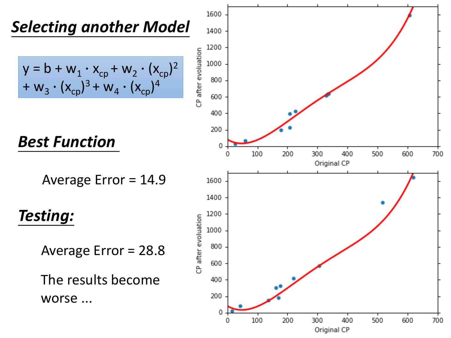
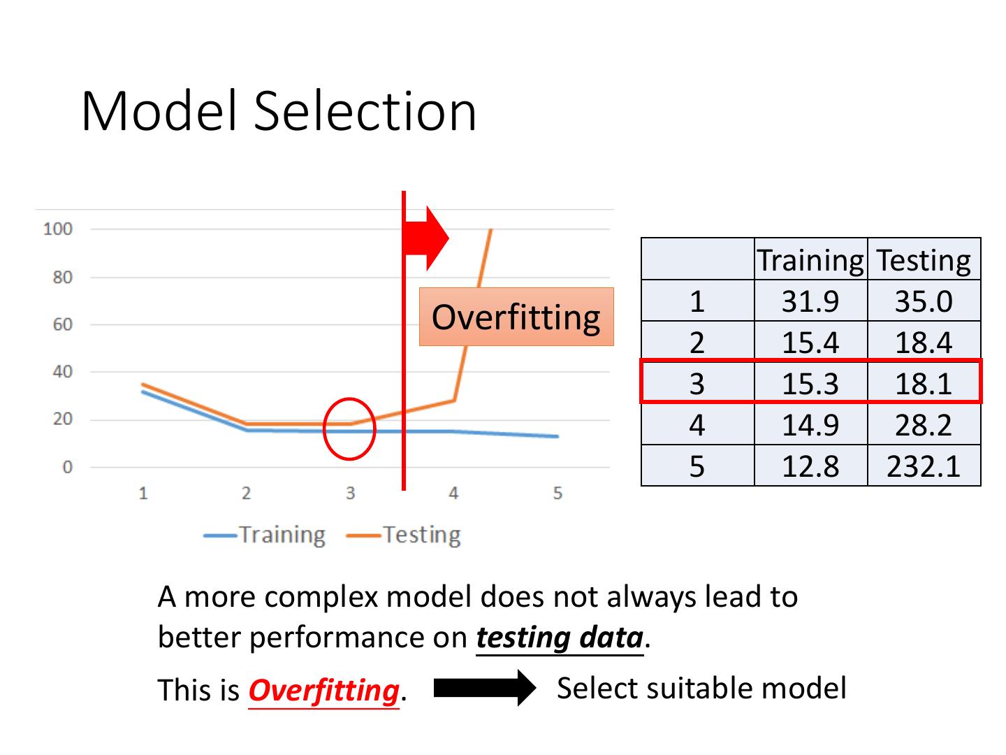
24 .Selecting another Model y = b + w1 ∙ xcp + w2 ∙ (xcp)2 + w3 ∙ (xcp)3 + w4 ∙ (xcp)4 Best Function Average Error = 14.9 Testing: Average Error = 28.8 The results become worse ... 

25 .Selecting another Model y = b + w1 ∙ xcp + w2 ∙ (xcp)2 + w3 ∙ (xcp)3 + w4 ∙ (xcp)4 + w5 ∙ (xcp)5 Best Function Average Error = 12.8 Testing: Average Error = 232.1 The results are so bad. 

26 . Training Data Model Selection 1. y = b + w ∙ xcp 2. y = b + w1 ∙ xcp + w2 ∙ (xcp)2 y = b + w1 ∙ xcp + w2 ∙ (xcp)2 3. + w3 ∙ (xcp)3 y = b + w1 ∙ xcp + w2 ∙ (xcp)2 4. + w3 ∙ (xcp)3 + w4 ∙ (xcp)4 y = b + w1 ∙ xcp + w2 ∙ (xcp)2 A more complex model yields 5. + w3 ∙ (xcp)3 + w4 ∙ (xcp)4 lower error on training data. + w5 ∙ (xcp)5 If we can truly find the best function 

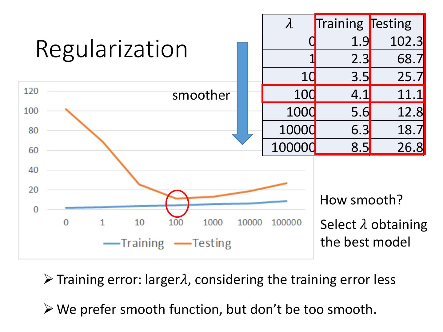
27 .Model Selection Training Testing 1 31.9 35.0 Overfitting 2 15.4 18.4 3 15.3 18.1 4 14.9 28.2 5 12.8 232.1 A more complex model does not always lead to better performance on testing data. This is Overfitting. Select suitable model 

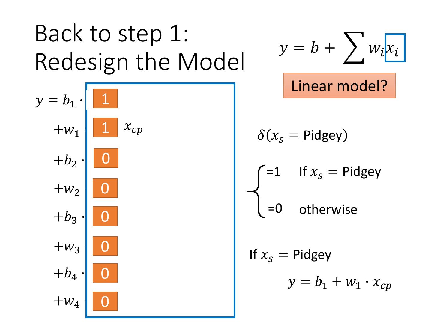
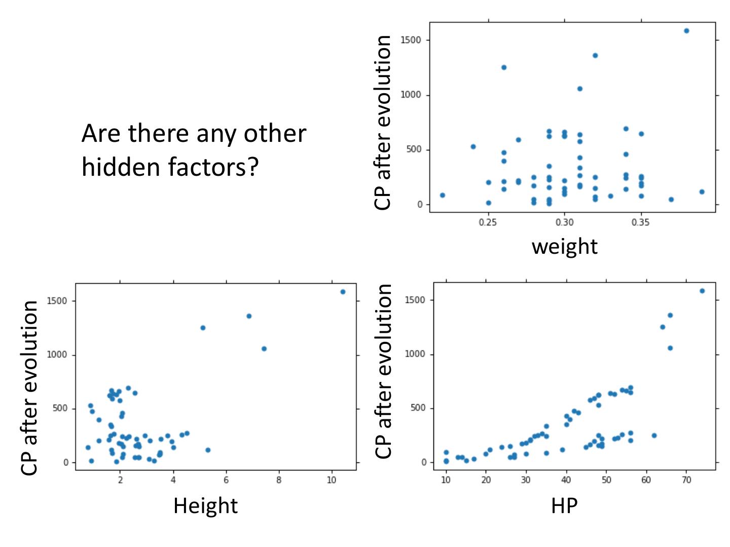
28 .Let’s collect more data There is some hidden factors not considered in the previous model …… 

29 .What are the hidden factors? Eevee Pidgey Weedle Caterpie