Gradient Descent

1 .Gradient Descent 

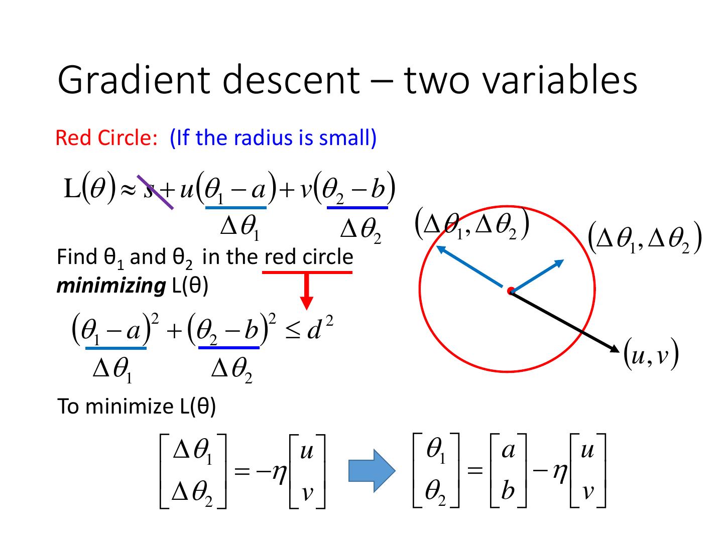
2 .Review: Gradient Descent • In step 3, we have to solve the following optimization problem: 𝜃 ∗ = arg min 𝐿 𝜃 L: loss function 𝜃: parameters 𝜃 Suppose that θ has two variables {θ1, θ2} 0 𝜃 𝜕𝐿 𝜃1 Τ𝜕𝜃1 Randomly start at 𝜃 0 = 10 𝛻𝐿 𝜃 = 𝜃2 𝜕𝐿 𝜃2 Τ𝜕𝜃2 𝜃11 𝜃10 𝜕𝐿 𝜃10 Τ𝜕𝜃1 1 = 0 −𝜂 0 Τ 𝜃 1 = 𝜃 0 − 𝜂𝛻𝐿 𝜃 0 𝜃2 𝜃2 𝜕𝐿 𝜃2 𝜕𝜃2 𝜃12 𝜃11 𝜕𝐿 𝜃11 Τ𝜕𝜃1 2 = 1 −𝜂 𝜃 2 = 𝜃 1 − 𝜂𝛻𝐿 𝜃 1 𝜃2 𝜃2 𝜕𝐿 𝜃21 Τ𝜕𝜃2 

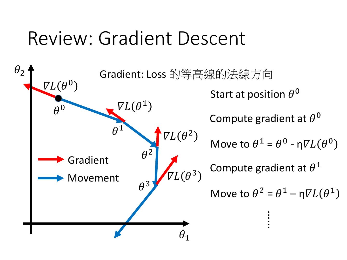
3 . Review: Gradient Descent 𝜃2 Gradient: Loss 的等高線的法線方向 𝛻𝐿 𝜃 0 Start at position 𝜃 0 𝜃 0 𝛻𝐿 𝜃 1 Compute gradient at 𝜃 0 𝜃1 𝛻𝐿 𝜃 2 Move to 𝜃 1 = 𝜃 0 - η𝛻𝐿 𝜃 0 Gradient 𝜃2 Compute gradient at 𝜃 1 Movement 𝛻𝐿 𝜃 3 𝜃3 Move to 𝜃 2 = 𝜃 1 – η𝛻𝐿 𝜃 1 …… 𝜃1 

4 .Gradient Descent Tip 1: Tuning your learning rates 

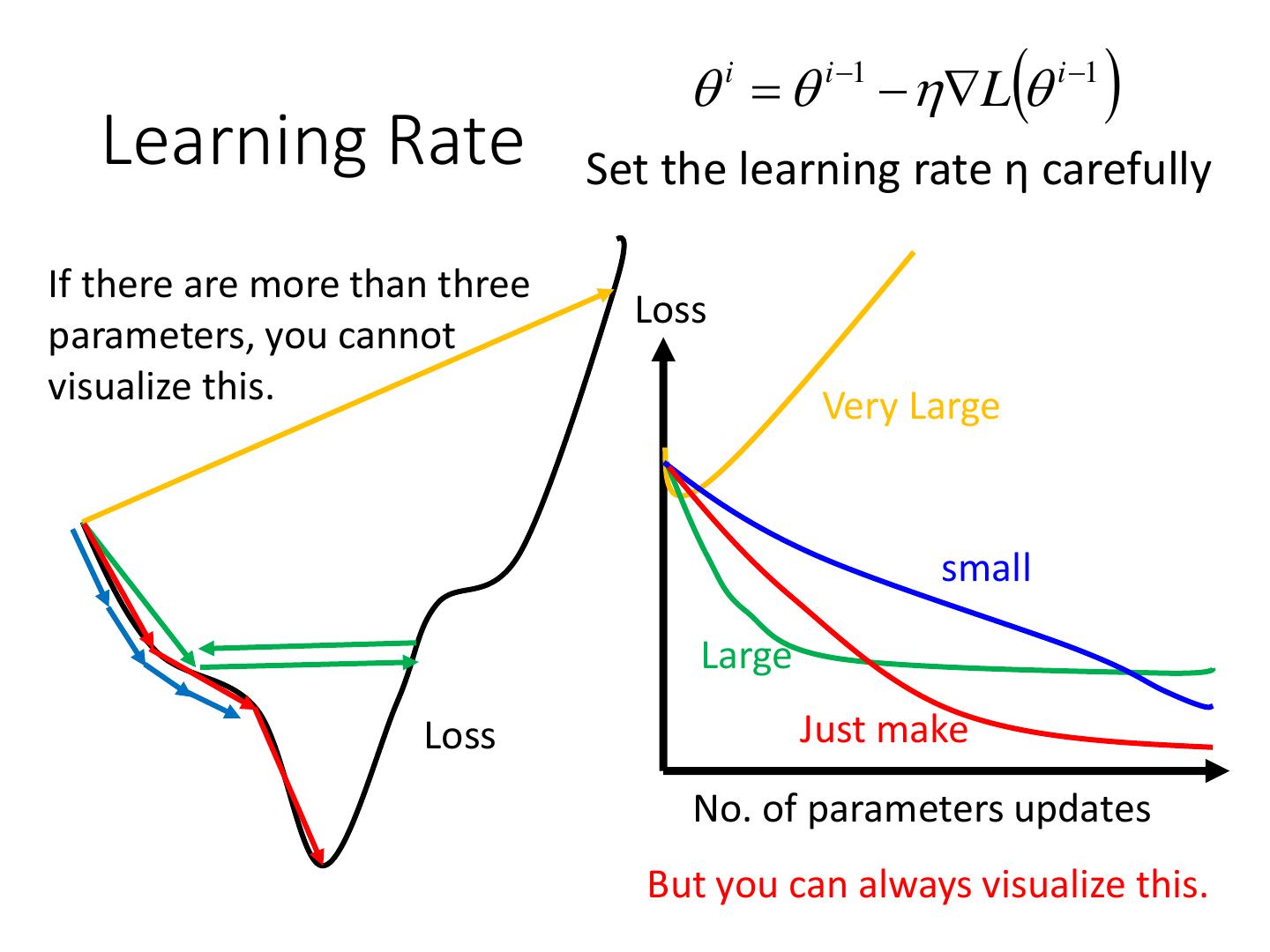
5 .  i i 1    L  i 1 Learning Rate Set the learning rate η carefully If there are more than three Loss parameters, you cannot visualize this. Very Large small Large Loss Just make No. of parameters updates But you can always visualize this. 

6 .Adaptive Learning Rates • Popular & Simple Idea: Reduce the learning rate by some factor every few epochs. • At the beginning, we are far from the destination, so we use larger learning rate • After several epochs, we are close to the destination, so we reduce the learning rate • E.g. 1/t decay: 𝜂 𝑡 = 𝜂 Τ 𝑡 + 1 • Learning rate cannot be one-size-fits-all • Giving different parameters different learning rates 

7 . 𝜂 𝑡 𝜕𝐿 𝜃 Adagrad 𝜂𝑡 = 𝑔𝑡 = 𝑡+1 𝜕𝑤 • Divide the learning rate of each parameter by the root mean square of its previous derivatives Vanilla Gradient descent 𝑤 𝑡+1 ← 𝑤 𝑡 − 𝜂 𝑡 𝑔𝑡 w is one parameters Adagrad 𝑡 𝜎 𝑡 : root mean square of 𝜂 𝑤 𝑡+1 ← 𝑤 𝑡 − 𝑡 𝑔𝑡 the previous derivatives of 𝜎 parameter w Parameter dependent 

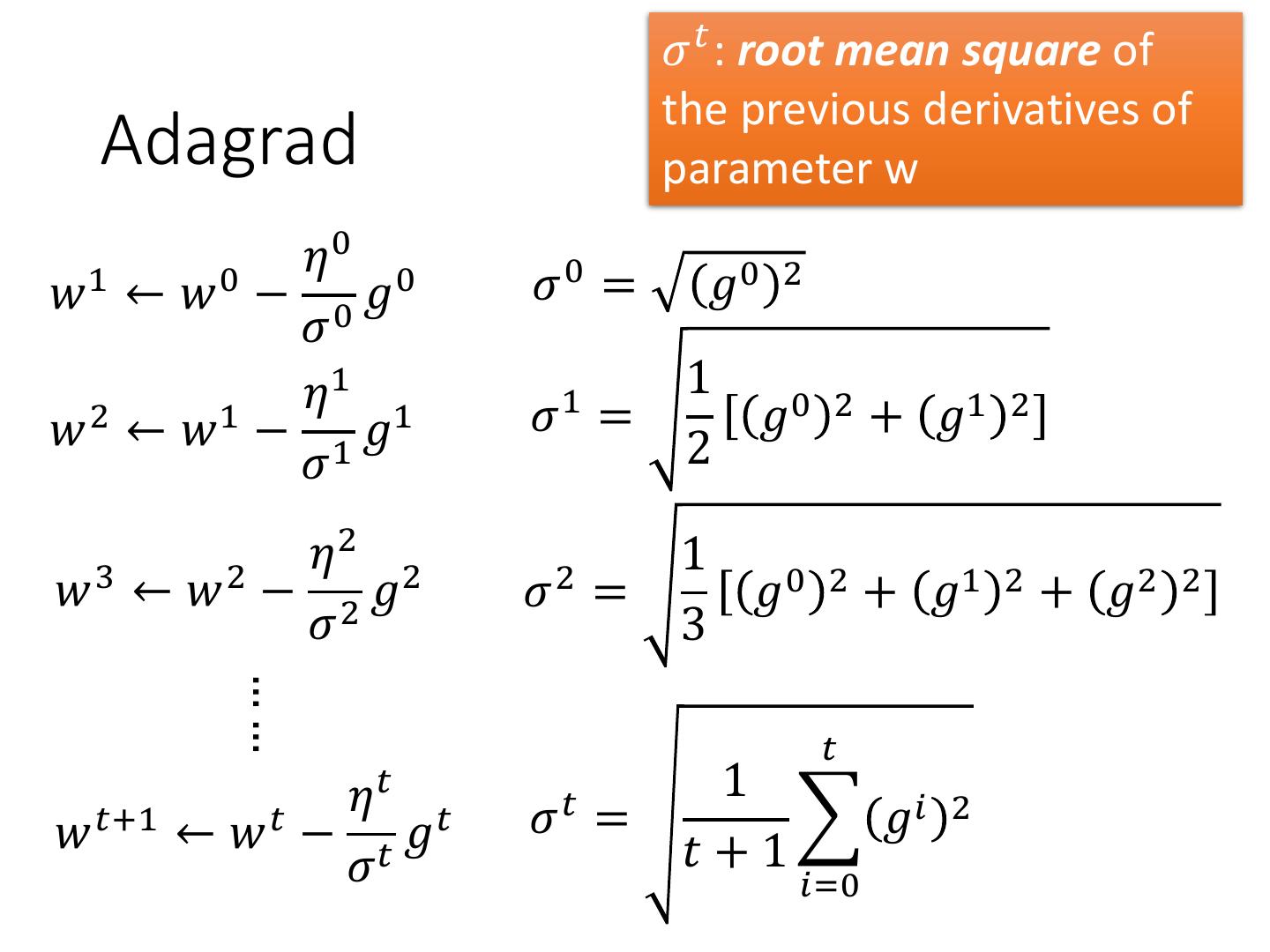
8 . 𝜎 𝑡 : root mean square of the previous derivatives of Adagrad parameter w 𝜂 0 𝑤 1 ← 𝑤 0 − 0 𝑔0 𝜎0 = 𝑔0 2 𝜎 𝜂 1 1 1 𝑤 2 ← 𝑤 1 − 1 𝑔1 𝜎 = 𝑔0 2 + 𝑔1 2 𝜎 2 𝜂 2 1 𝑤 3 ← 𝑤 2 − 2 𝑔2 𝜎2 = 𝑔0 2 + 𝑔1 2 + 𝑔2 2 𝜎 3 …… 𝑡 𝜂 𝑡 1 𝑤 𝑡+1 ← 𝑤 𝑡 − 𝑡 𝑔𝑡 𝜎𝑡 = ෍ 𝑔𝑖 2 𝜎 𝑡+1 𝑖=0 

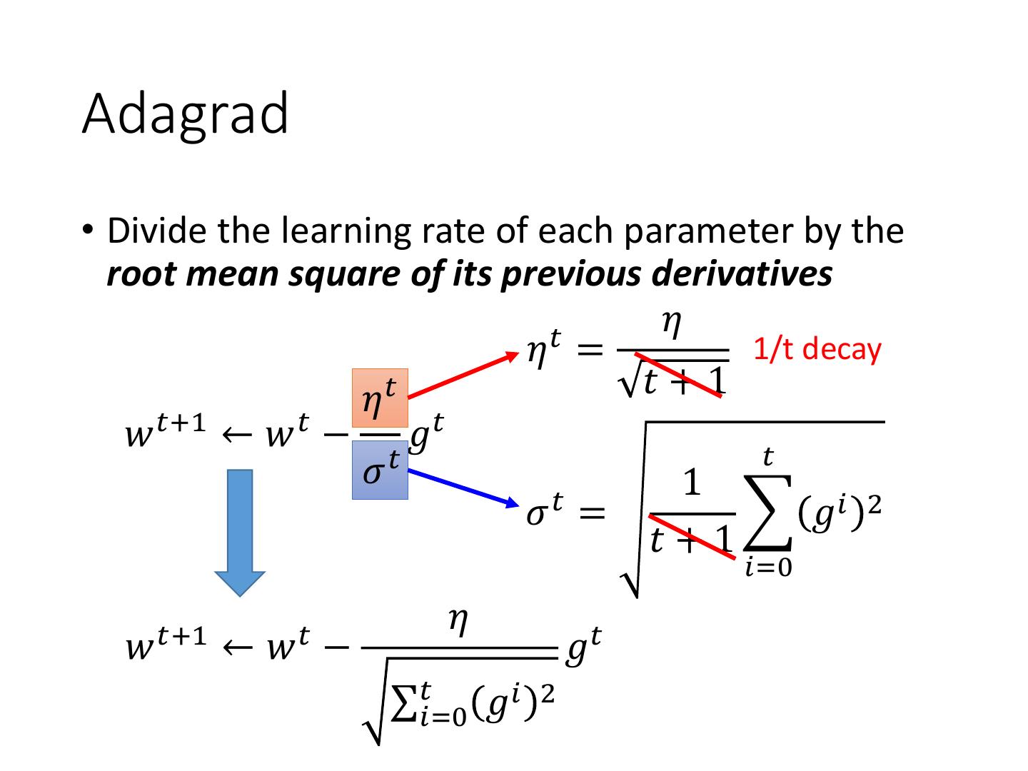
9 .Adagrad • Divide the learning rate of each parameter by the root mean square of its previous derivatives 𝑡 𝜂 𝜂 = 1/t decay 𝜂𝜂𝑡 𝑡 + 1 𝑡+1 𝑤 ← 𝑤 − 𝑡 𝑔𝑡 𝑡 𝜎 𝜎𝑡 𝑡 𝑡 1 𝜎 = ෍ 𝑔𝑖 2 𝑡+1 𝑖=0 𝜂 𝑤 𝑡+1 ← 𝑤𝑡 − 𝑔𝑡 σ𝑡𝑖=0 𝑔𝑖 2 

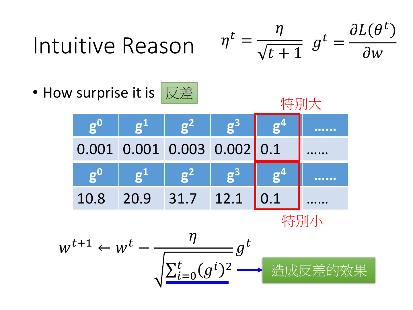
10 . 𝜂 𝜕𝐿 𝜃 𝑡 Contradiction? 𝜂𝑡 = 𝑔𝑡 = 𝑡+1 𝜕𝑤 Vanilla Gradient descent 𝑡+1 𝑡 𝑡 𝑡 Larger gradient, 𝑤 ←𝑤 −𝜂 𝑔 larger step Adagrad Larger gradient, 𝜂 larger step 𝑤 𝑡+1 ← 𝑤𝑡 − 𝑔𝑡 σ𝑡𝑖=0 𝑔𝑖 2 Larger gradient, smaller step 

11 . 𝜂 𝜕𝐿 𝜃 𝑡 𝜂𝑡 = 𝑔𝑡 = Intuitive Reason 𝑡+1 𝜕𝑤 • How surprise it is 反差 特別大 g0 g1 g2 g3 g4 …… 0.001 0.001 0.003 0.002 0.1 …… g0 g1 g2 g3 g4 …… 10.8 20.9 31.7 12.1 0.1 …… 特別小 𝑡+1 𝑡 𝜂 𝑤 ←𝑤 − 𝑔𝑡 σ𝑡𝑖=0 𝑔𝑖 2 造成反差的效果 

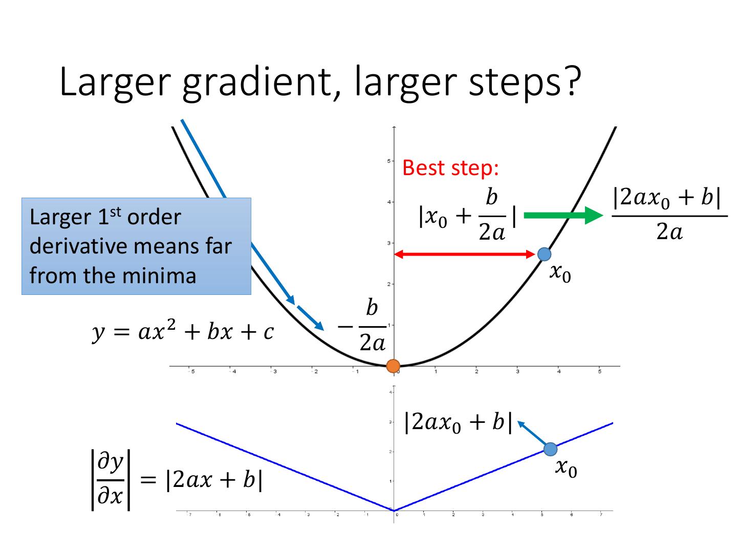
12 . Larger gradient, larger steps? Best step: 𝑏 |2𝑎𝑥0 + 𝑏| 1st Larger order |𝑥0 + | 2𝑎 2𝑎 derivative means far from the minima 𝑥0 𝑏 𝑦 = 𝑎𝑥 2 + 𝑏𝑥 + 𝑐 − 2𝑎 |2𝑎𝑥0 + 𝑏| 𝜕𝑦 𝑥0 = |2𝑎𝑥 + 𝑏| 𝜕𝑥 

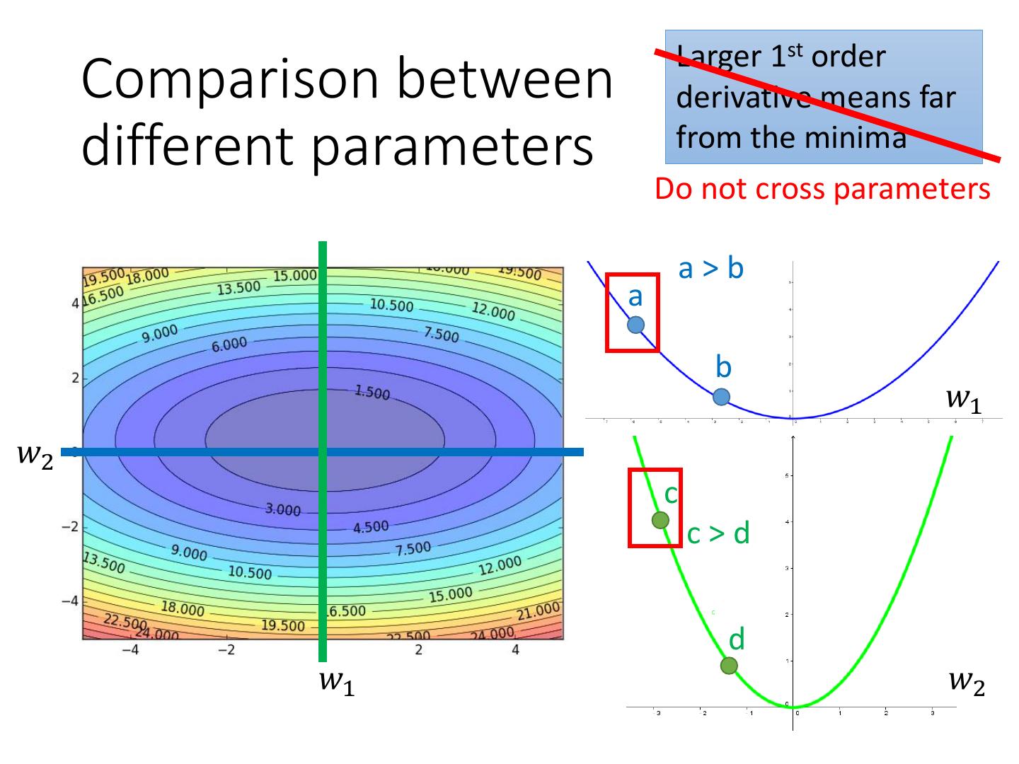
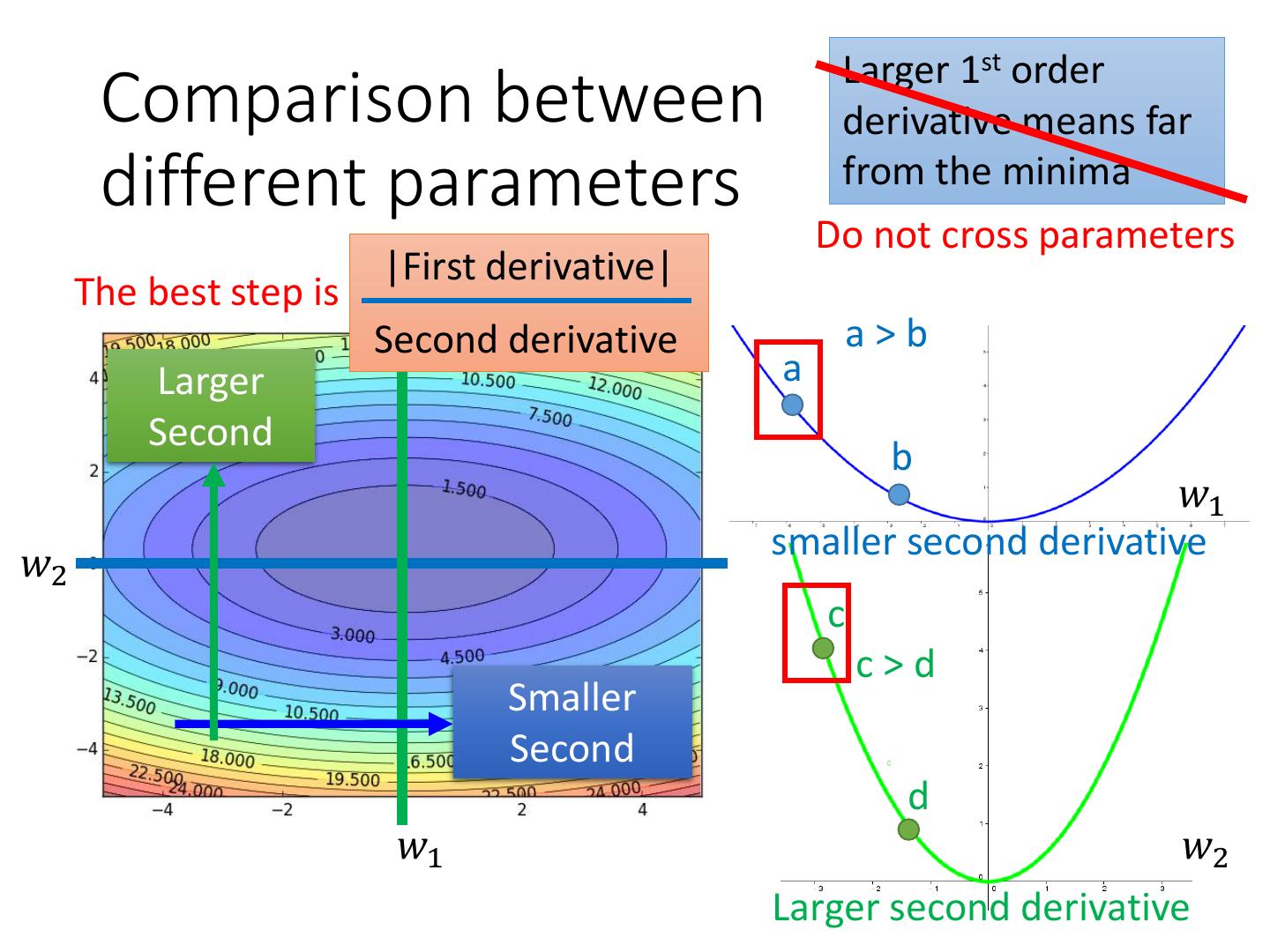
13 . Larger 1st order Comparison between derivative means far different parameters from the minima Do not cross parameters a>b a b 𝑤1 𝑤2 c c>d d 𝑤1 𝑤2 

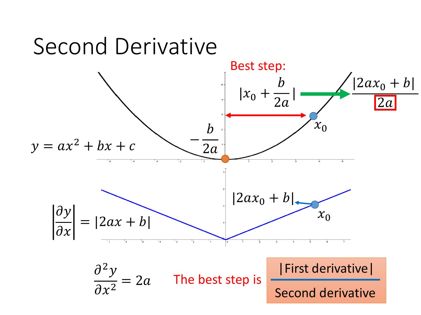
14 .Second Derivative Best step: 𝑏 |2𝑎𝑥0 + 𝑏| |𝑥0 + | 2𝑎 2𝑎 𝑏 𝑥0 𝑦 = 𝑎𝑥 2 + 𝑏𝑥 + 𝑐 − 2𝑎 |2𝑎𝑥0 + 𝑏| 𝜕𝑦 𝑥0 = |2𝑎𝑥 + 𝑏| 𝜕𝑥 𝜕2𝑦 |First derivative| 2 = 2𝑎 The best step is 𝜕𝑥 Second derivative 

15 . Larger 1st order Comparison between derivative means far different parameters from the minima Do not cross parameters |First derivative| The best step is Second derivative a>b Larger a Second b 𝑤1 smaller second derivative 𝑤2 c c>d Smaller Second d 𝑤1 𝑤2 Larger second derivative 

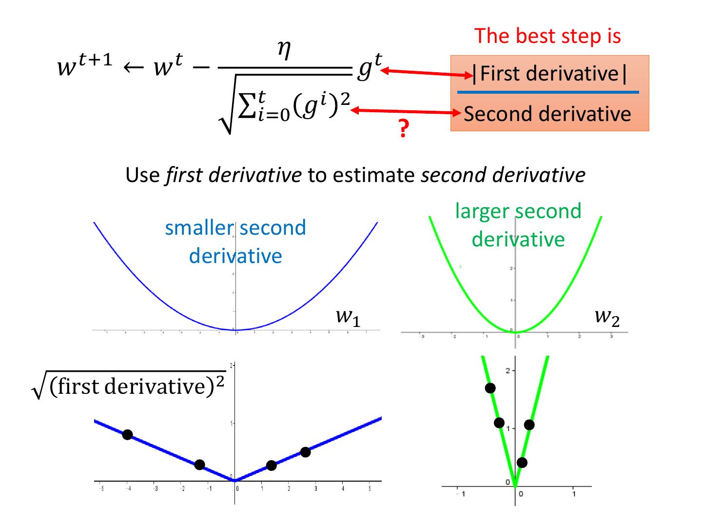
16 . The best step is 𝜂 𝑤 𝑡+1 ← 𝑤 𝑡 − 𝑔𝑡 |First derivative| σ𝑡𝑖=0 𝑔𝑖 2 Second derivative ? Use first derivative to estimate second derivative larger second smaller second derivative derivative 𝑤1 𝑤2 first derivative 2 

17 .Gradient Descent Tip 2: Stochastic Gradient Descent Make the training faster 

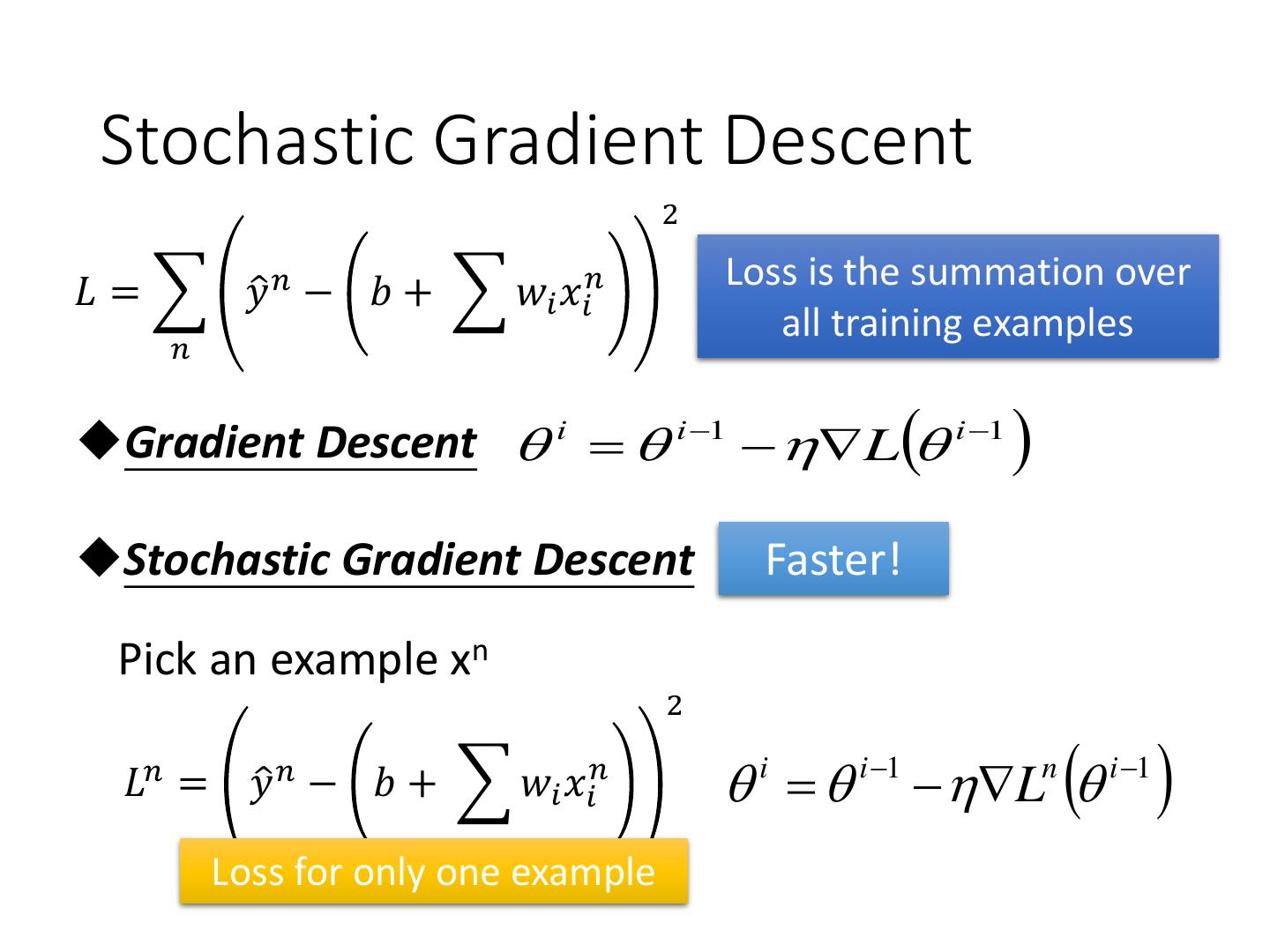
18 . Stochastic Gradient Descent 2 𝐿 = ෍ 𝑦ො 𝑛 − 𝑏 + ෍ 𝑤𝑖 𝑥𝑖𝑛 Loss is the summation over all training examples 𝑛 Gradient Descent  i   i 1  L  i 1  Stochastic Gradient Descent Faster! Pick an example xn 2 𝐿𝑛 = 𝑦ො 𝑛 − 𝑏 + ෍ 𝑤𝑖 𝑥𝑖𝑛  i   i 1  Ln  i 1  Loss for only one example 

19 .• Demo 

20 .Stochastic Gradient Descent Stochastic Gradient Descent Gradient Descent Update for each example Update after seeing all If there are 20 examples, examples 20 times faster. See all See only one examples example See all examples 

21 .Gradient Descent Tip 3: Feature Scaling 

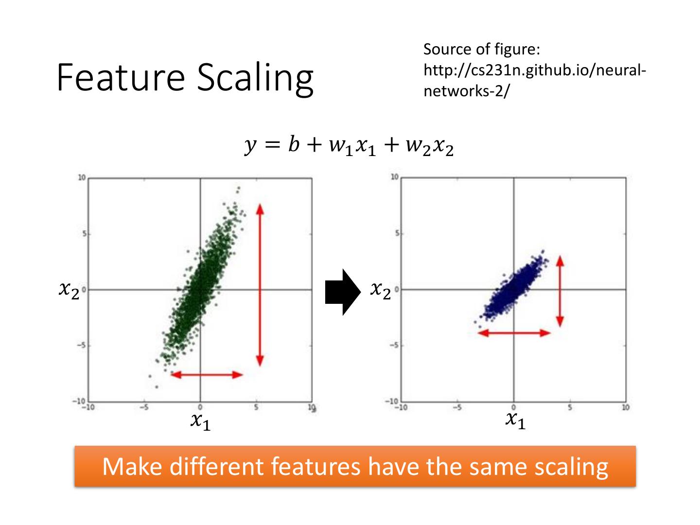
22 . Source of figure: Feature Scaling http://cs231n.github.io/neural- networks-2/ 𝑦 = 𝑏 + 𝑤1 𝑥1 + 𝑤2 𝑥2 𝑥2 𝑥2 𝑥1 𝑥1 Make different features have the same scaling 

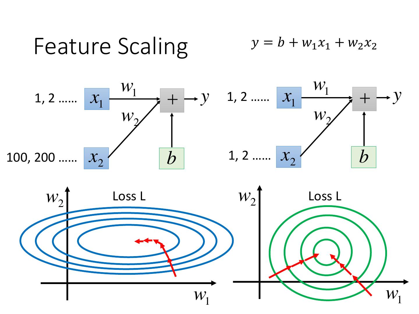
23 . 𝑦 = 𝑏 + 𝑤1 𝑥1 + 𝑤2 𝑥2 Feature Scaling w1 w1 1, 2 …… x1  y 1, 2 …… x1  y w2 w2 100, 200 …… x2 b 1, 2 …… x2 b w2 Loss L w2 Loss L w1 w1 

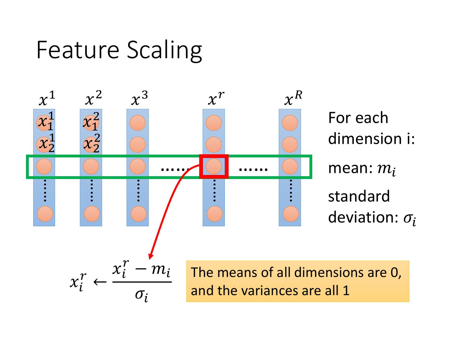
24 .Feature Scaling 𝑥1 𝑥2 𝑥3 𝑥𝑟 𝑥𝑅 𝑥11 𝑥12 For each 𝑥21 𝑥22 dimension i: …… …… mean: 𝑚𝑖 …… …… …… …… …… standard deviation: 𝜎𝑖 𝑟 𝑟 𝑥𝑖 − 𝑚𝑖 The means of all dimensions are 0, 𝑥𝑖 ← 𝜎𝑖 and the variances are all 1 

25 .Gradient Descent Theory 

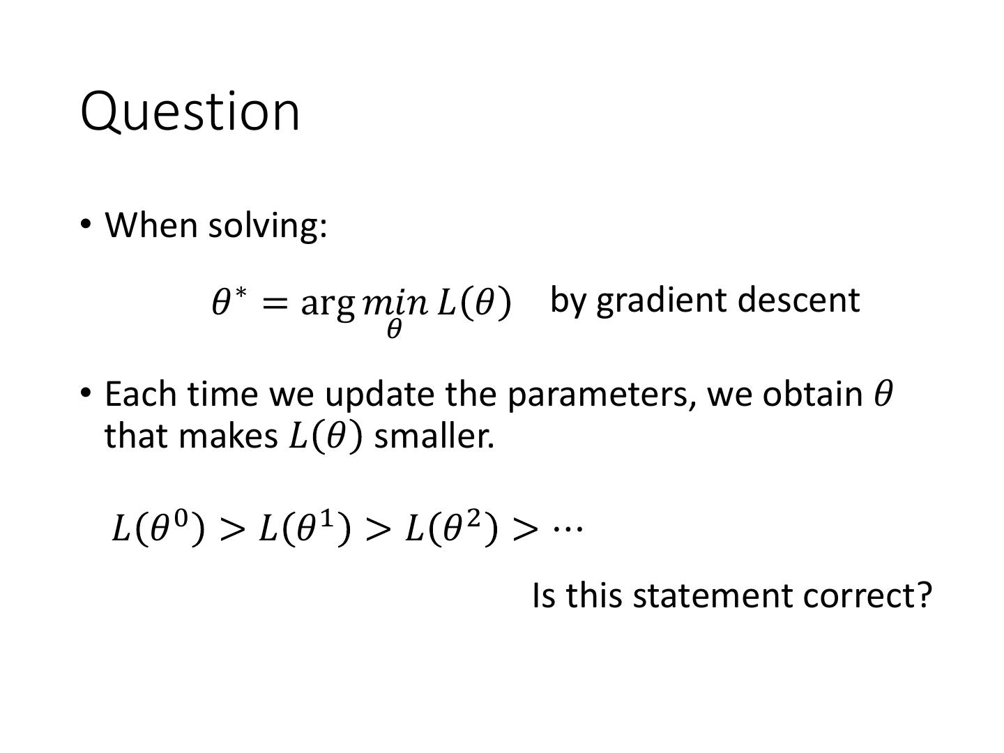
26 .Question • When solving: 𝜃 ∗ = arg 𝑚𝑖𝑛 𝐿 𝜃 by gradient descent 𝜃 • Each time we update the parameters, we obtain 𝜃 that makes 𝐿 𝜃 smaller. 𝐿 𝜃 0 > 𝐿 𝜃1 > 𝐿 𝜃 2 > ⋯ Is this statement correct? 

27 .Warning of Math 

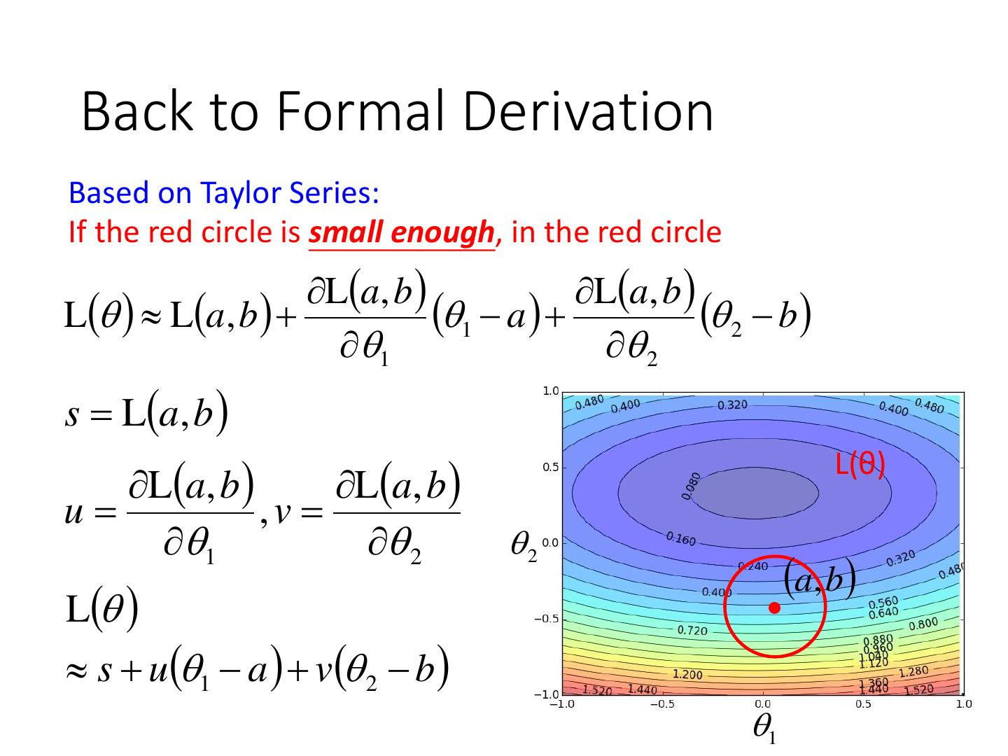
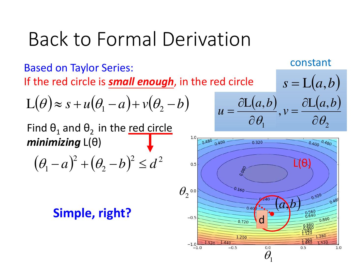
28 . Formal Derivation • Suppose that θ has two variables {θ1, θ2} L(θ) 2 2 Given a point, we can 1 easily find the point with the smallest value 0 nearby. How? 1 

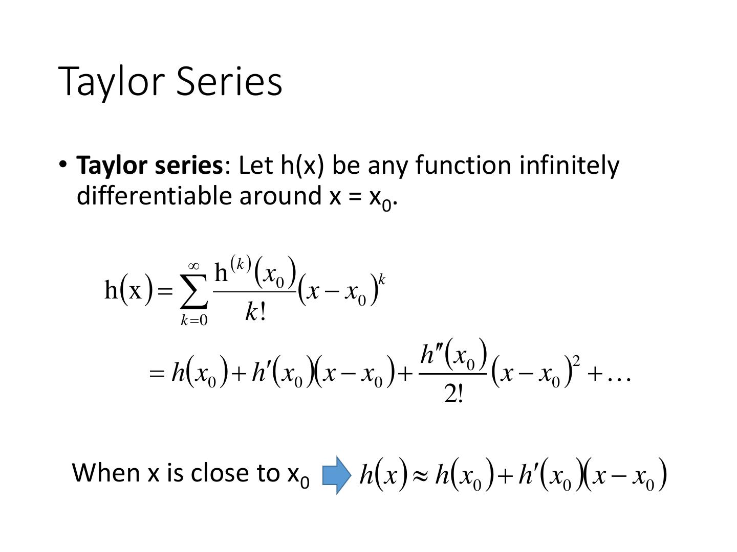
29 .Taylor Series • Taylor series: Let h(x) be any function infinitely differentiable around x = x0.  h k   x0  h x    x  x0 k k 0 k! h x0   h x0   h  x0  x  x0    x  x0    2 2! When x is close to x0 h x   h x0   h x0  x  x0 