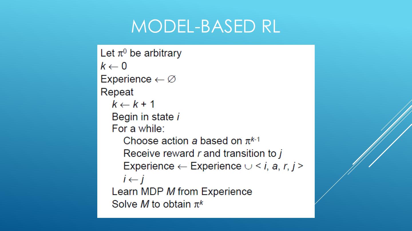
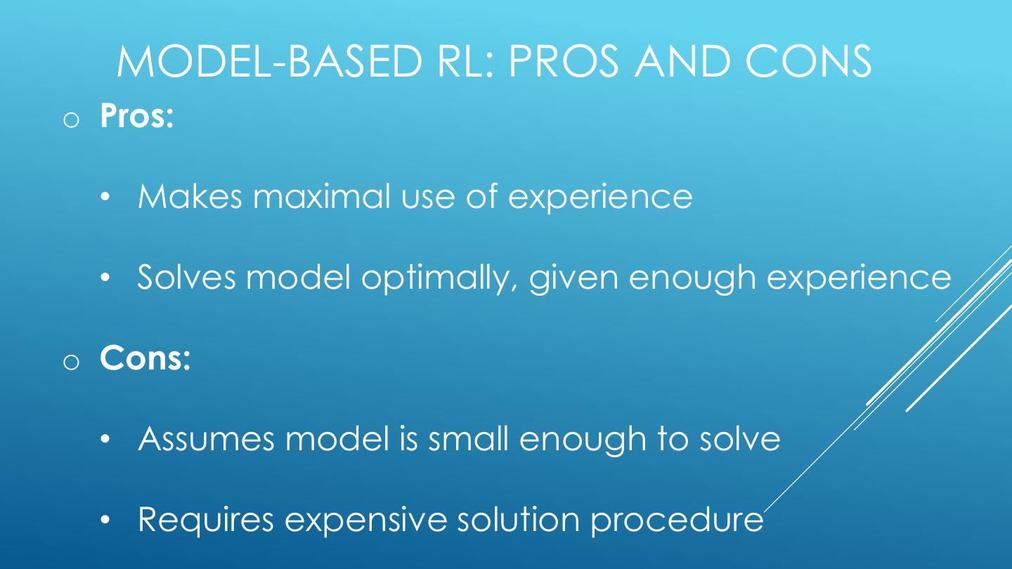
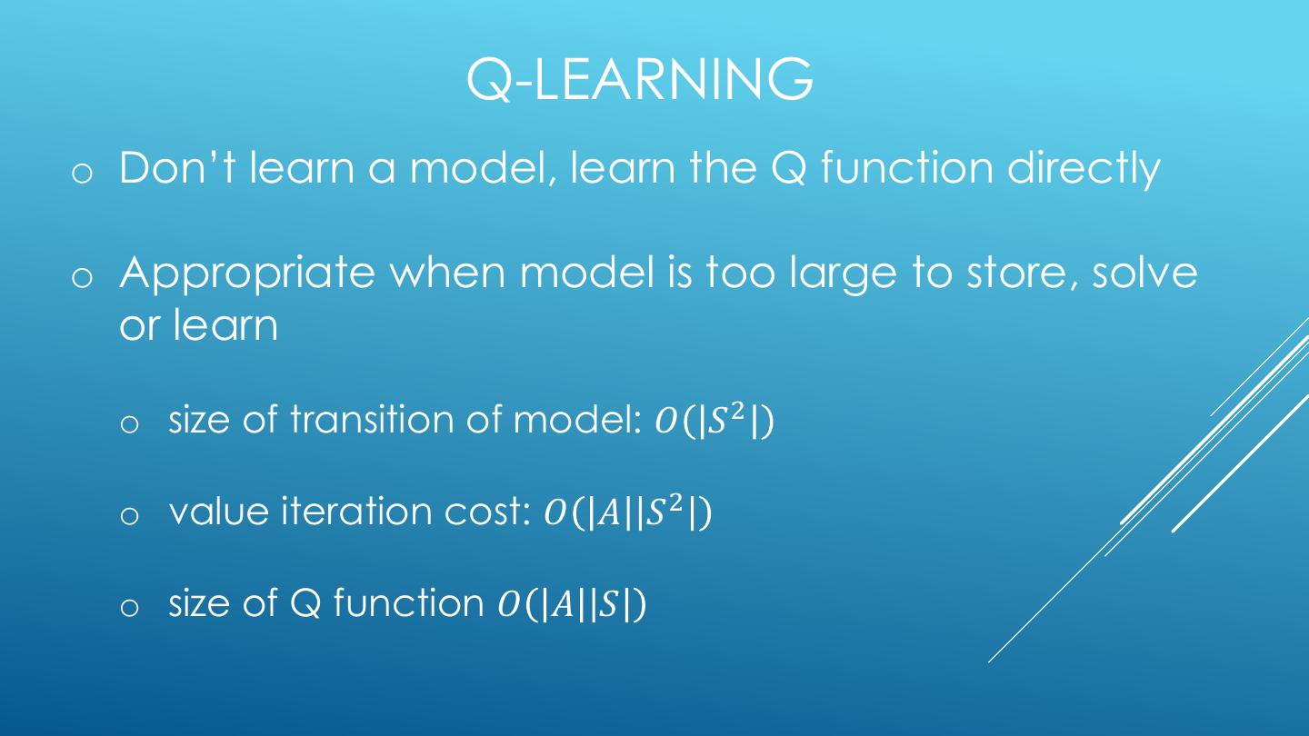
Towards Q-learning

1 .TOWARDS Q-LEARNING 

2 . CS181 course at Harvard University: CS181 Intelligent Machines: Perception, Learning and REFERENCES  Uncertainty, Sarah Finney, Spring 2009  CS181 Intelligent Machines: Perception, Learning and The material for this Uncertainty, Prof. David C Brooks, Spring 2011 talk is primarily drawn from the slides, notes  CS181 – Machine Learning, Prof. Ryan P. Adams, Spring and lectures of these 2014. https://github.com/wihl/cs181-spring2014 courses:  CS181 – Machine Learning, Prof. David Parkes, Spring 2017. https://harvard-ml-courses.github.io/cs181-web-2017/ University of California, Berkeley CS188:  CS188 – Introduction to Artificial Intelligence, Profs. Dan Klein, Pieter Abbeel, et al. http://ai.berkeley.edu/home.html Stanford course CS229 :  CS229 – Machine Learning, Andrew Ng. https://see.stanford.edu/Course/CS229 

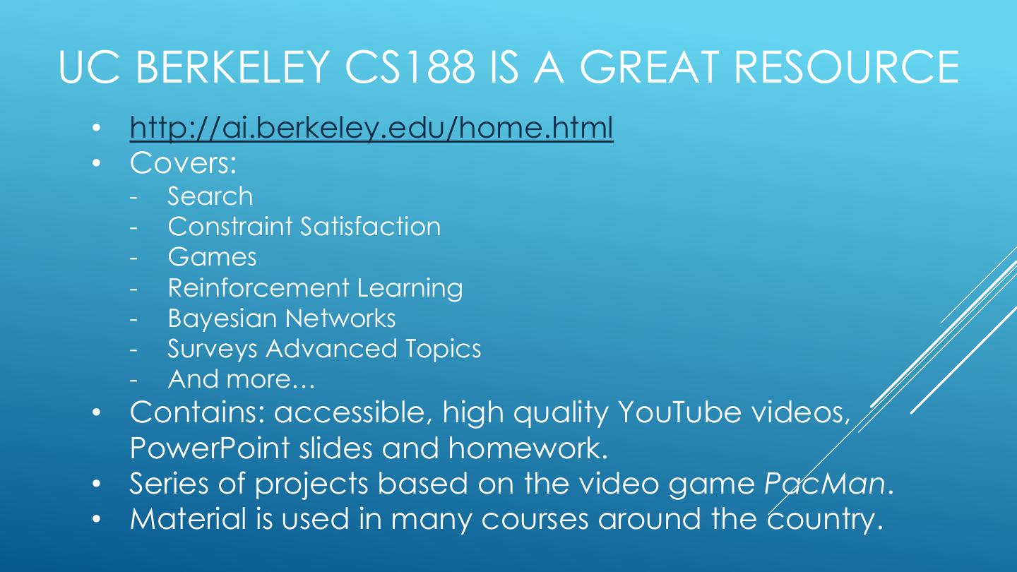
3 .UC BERKELEY CS188 IS A GREAT RESOURCE • http://ai.berkeley.edu/home.html • Covers: - Search - Constraint Satisfaction - Games - Reinforcement Learning - Bayesian Networks - Surveys Advanced Topics - And more… • Contains: accessible, high quality YouTube videos, PowerPoint slides and homework. • Series of projects based on the video game PacMan. • Material is used in many courses around the country. 

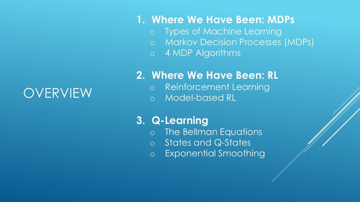
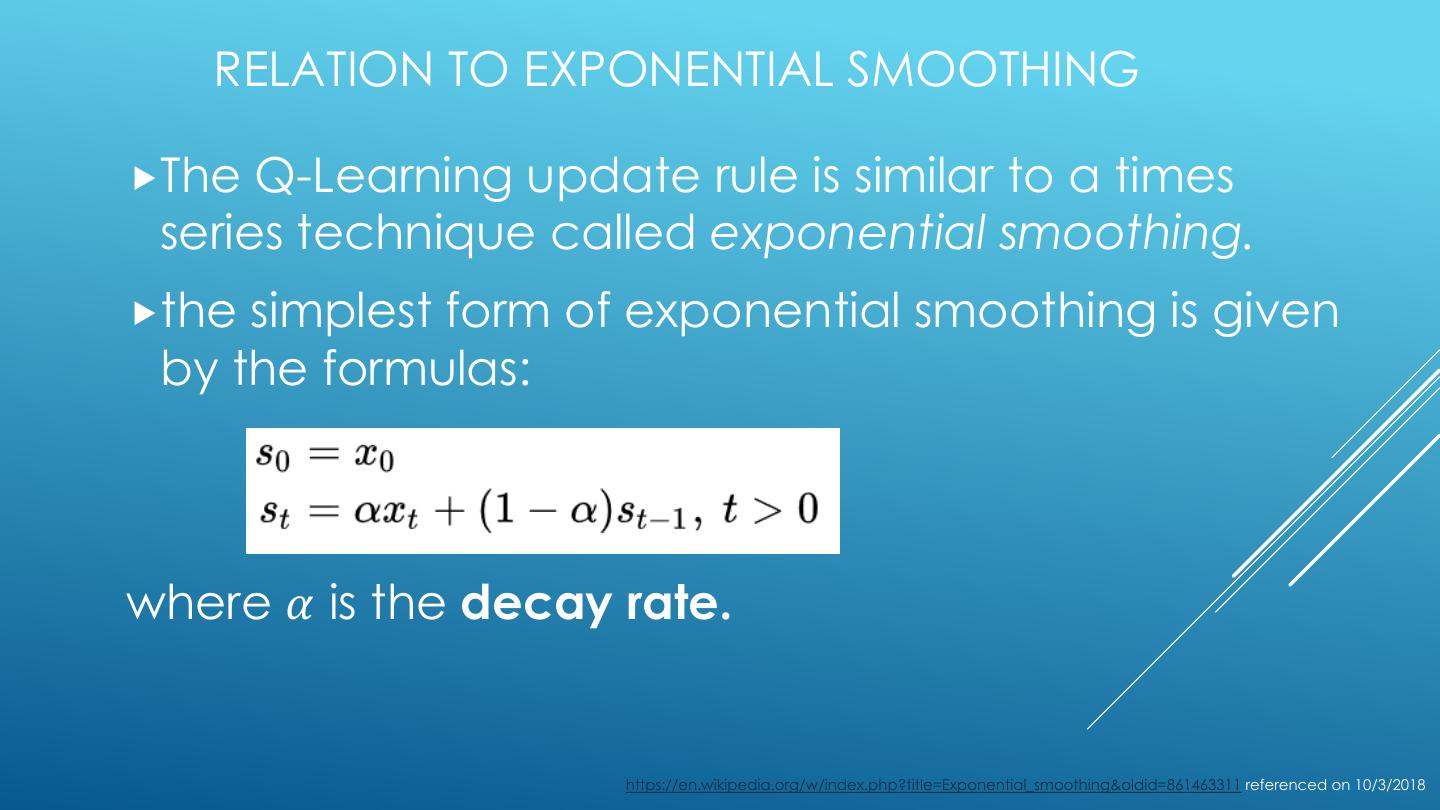
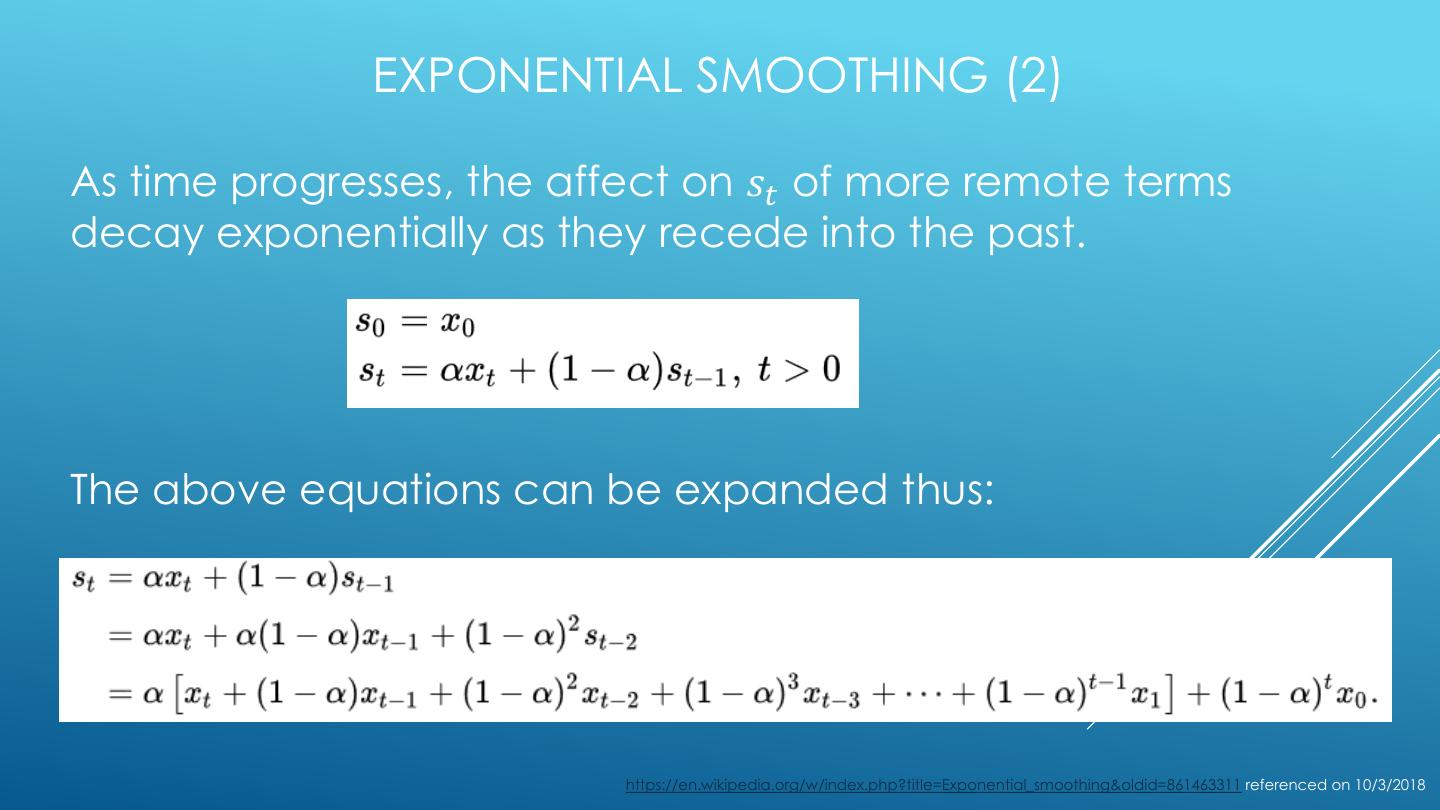
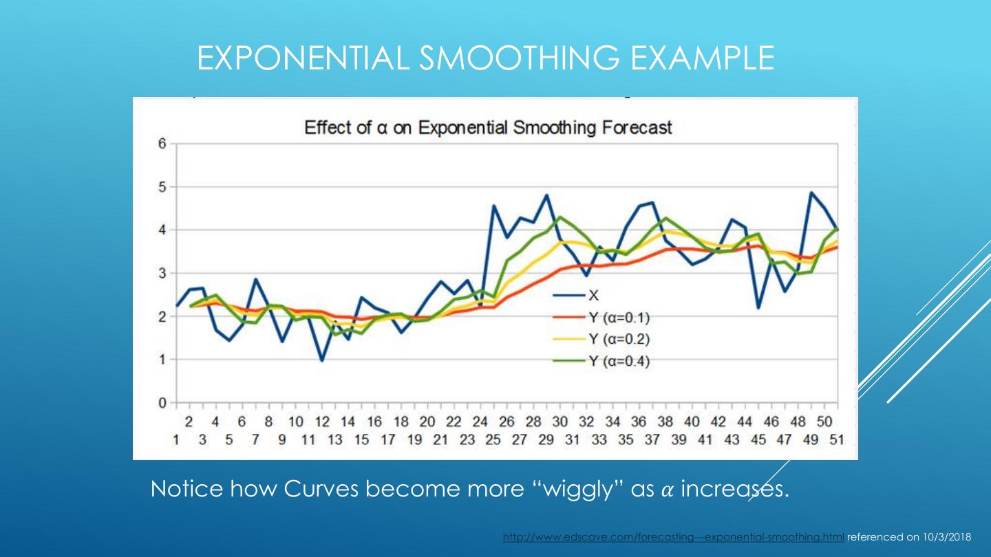
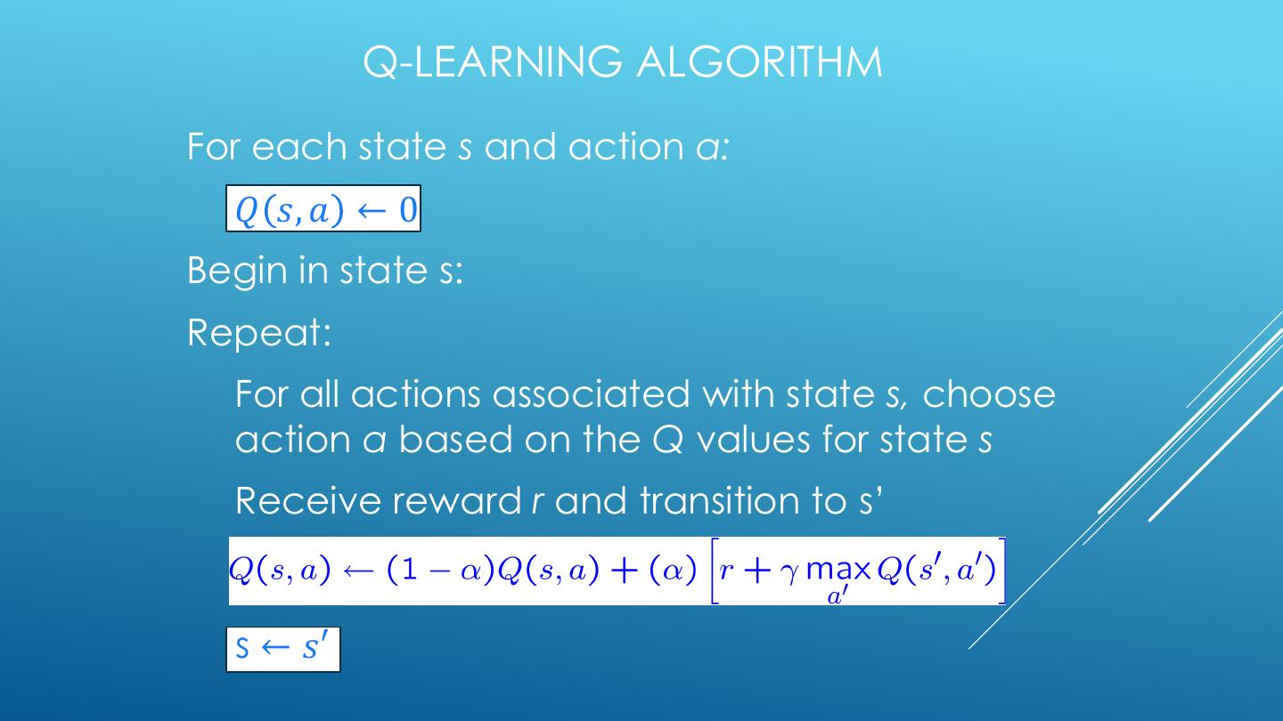
4 . 1. Where We Have Been: MDPs o Types of Machine Learning o Markov Decision Processes (MDPs) o 4 MDP Algorithms 2. Where We Have Been: RL o Reinforcement Learning OVERVIEW o Model-based RL 3. Q-Learning o The Bellman Equations o States and Q-States o Exponential Smoothing 

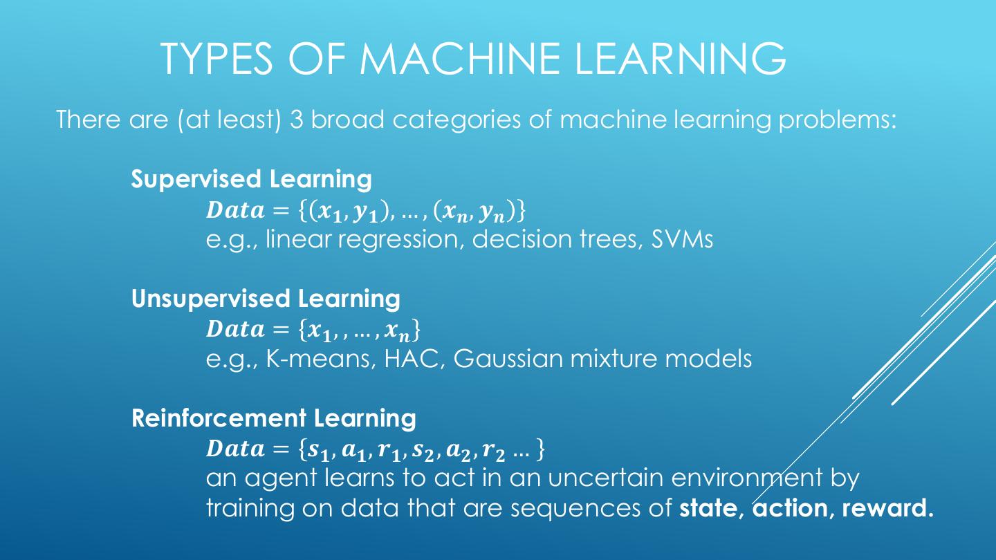
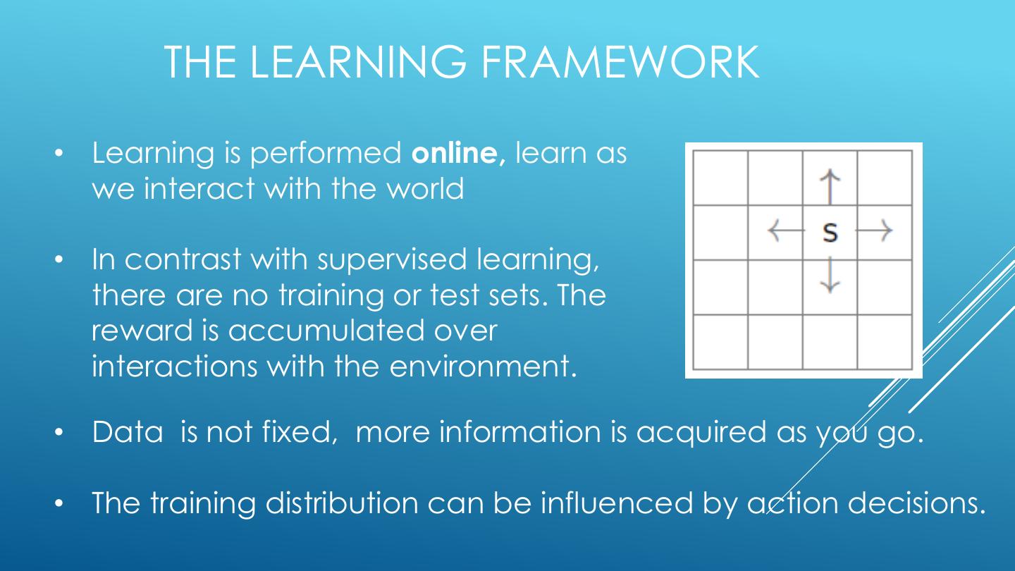
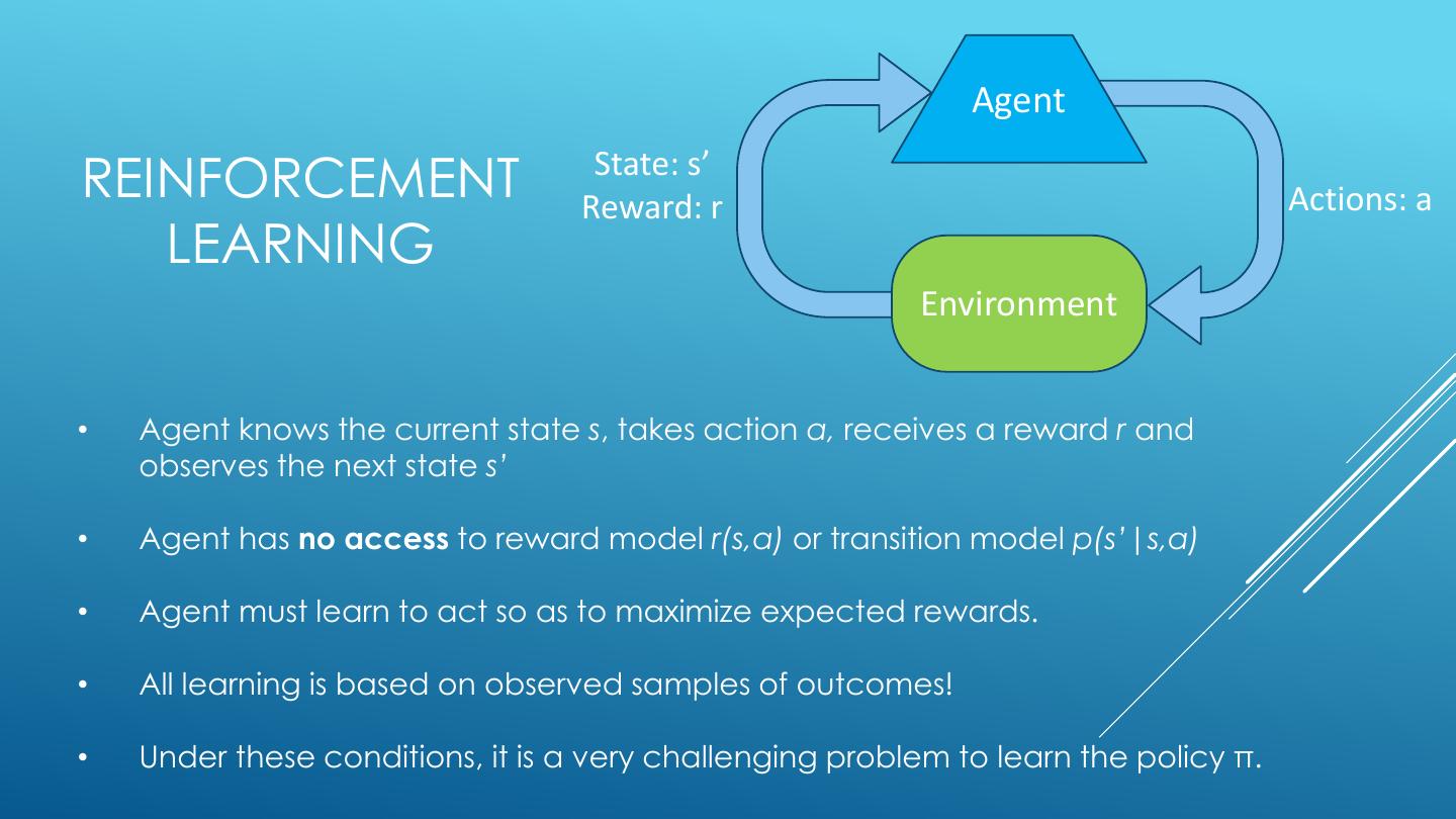
5 . TYPES OF MACHINE LEARNING There are (at least) 3 broad categories of machine learning problems: Supervised Learning 𝑫𝒂𝒕𝒂 = 𝒙𝟏 , 𝒚𝟏 , … , 𝒙𝒏 , 𝒚𝒏 e.g., linear regression, decision trees, SVMs Unsupervised Learning 𝑫𝒂𝒕𝒂 = 𝒙𝟏 , , … , 𝒙𝒏 e.g., K-means, HAC, Gaussian mixture models Reinforcement Learning 𝑫𝒂𝒕𝒂 = 𝒔𝟏 , 𝒂𝟏 , 𝒓𝟏 , 𝒔𝟐 , 𝒂𝟐 , 𝒓𝟐 … an agent learns to act in an uncertain environment by training on data that are sequences of state, action, reward. 

6 .MARKOV DECISION PROCESSES 

7 . MARKOV DECISION PROCESSES • Markov Decision Processes provide a mathematical framework for modeling decision making in situations where outcomes are partly random and partly under the control of a decision maker. • The initial analysis of MDPs assume complete knowledge of states, actions, rewards, transitions, and discounts. <https://en.wikipedia.org/w/index.php?title=Markov_decision_process&oldid=855934986> [accessed 11 September 2018] 

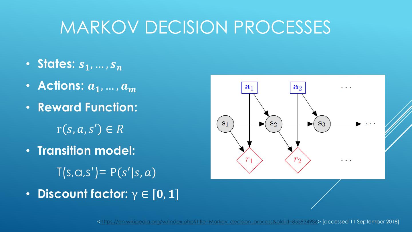
8 . MARKOV DECISION PROCESSES • States: 𝒔𝟏 , … , 𝒔𝒏 • Actions: 𝒂𝟏 , … , 𝒂𝒎 • Reward Function: r 𝑠, 𝑎, 𝑠′ ∈ 𝑅 • Transition model: T(s,a,s’)= P 𝑠′ 𝑠, 𝑎 • Discount factor: γ ∈ 𝟎, 𝟏 <https://en.wikipedia.org/w/index.php?title=Markov_decision_process&oldid=855934986> [accessed 11 September 2018] 

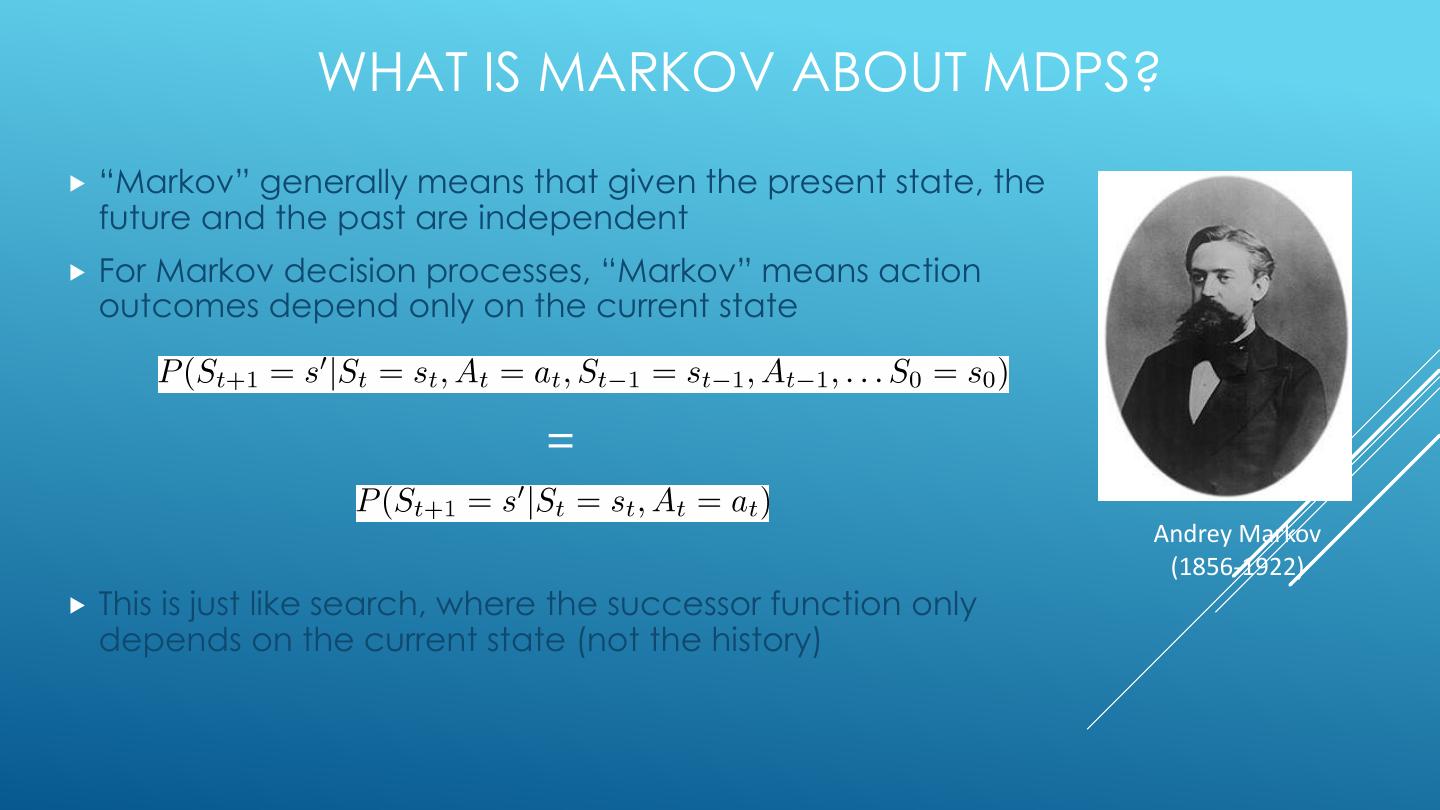
9 . WHAT IS MARKOV ABOUT MDPS?  “Markov” generally means that given the present state, the future and the past are independent  For Markov decision processes, “Markov” means action outcomes depend only on the current state = Andrey Markov (1856-1922)  This is just like search, where the successor function only depends on the current state (not the history) 

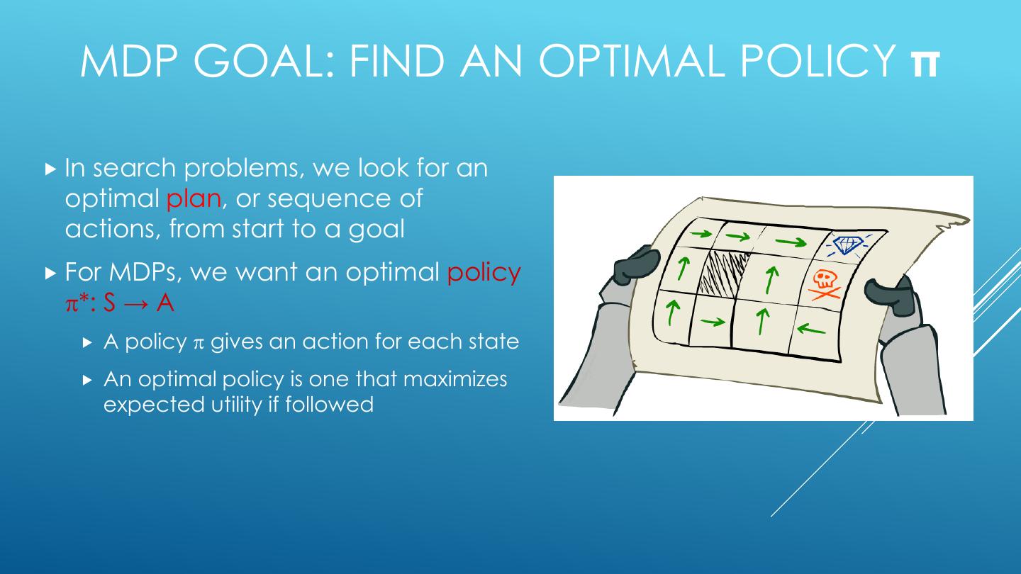
10 . MDP GOAL: FIND AN OPTIMAL POLICY π  Insearch problems, we look for an optimal plan, or sequence of actions, from start to a goal  For MDPs, we want an optimal policy *: S → A  A policy  gives an action for each state  An optimal policy is one that maximizes expected utility if followed 

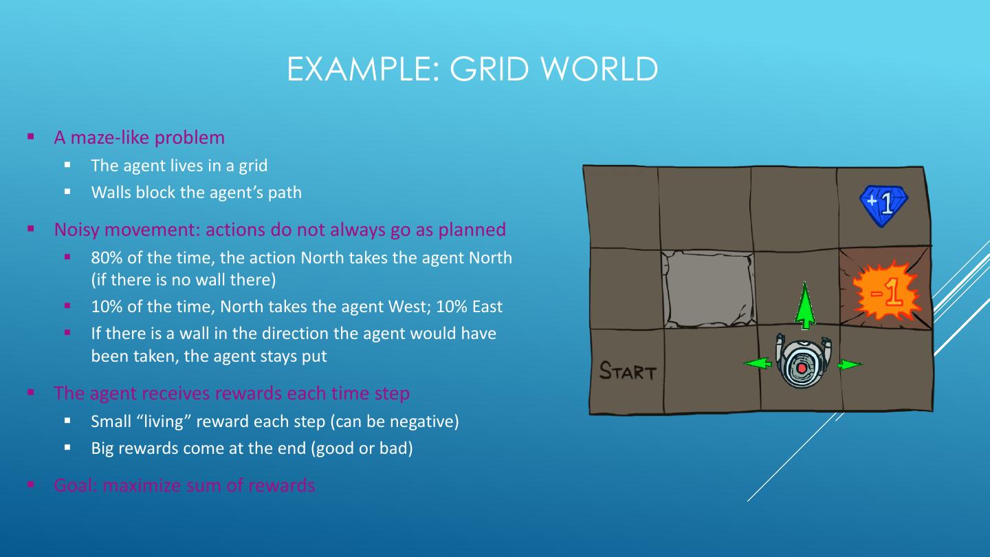
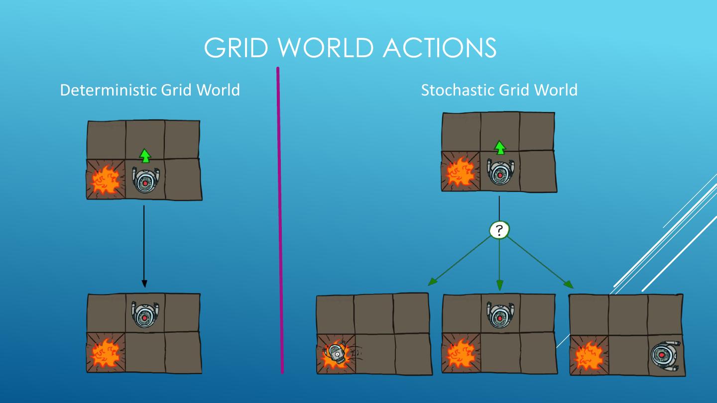
11 . EXAMPLE: GRID WORLD ▪ A maze-like problem ▪ The agent lives in a grid ▪ Walls block the agent’s path ▪ Noisy movement: actions do not always go as planned ▪ 80% of the time, the action North takes the agent North (if there is no wall there) ▪ 10% of the time, North takes the agent West; 10% East ▪ If there is a wall in the direction the agent would have been taken, the agent stays put ▪ The agent receives rewards each time step ▪ Small “living” reward each step (can be negative) ▪ Big rewards come at the end (good or bad) ▪ Goal: maximize sum of rewards 

12 . GRID WORLD ACTIONS Deterministic Grid World Stochastic Grid World 

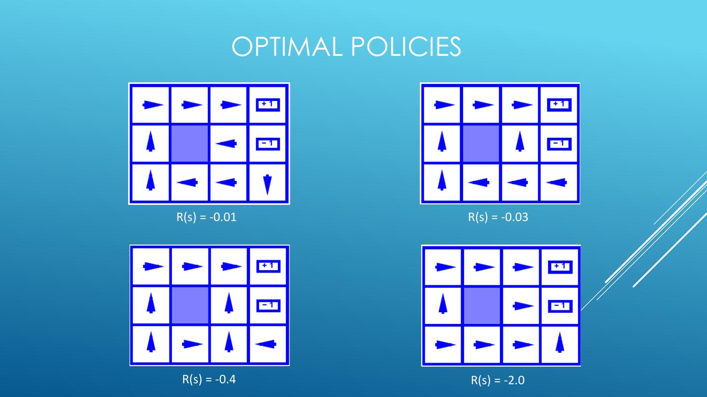
13 . OPTIMAL POLICIES R(s) = -0.01 R(s) = -0.03 R(s) = -0.4 R(s) = -2.0 

14 .MDP QUANTITIES AND THE BELLMAN EQUATIONS 

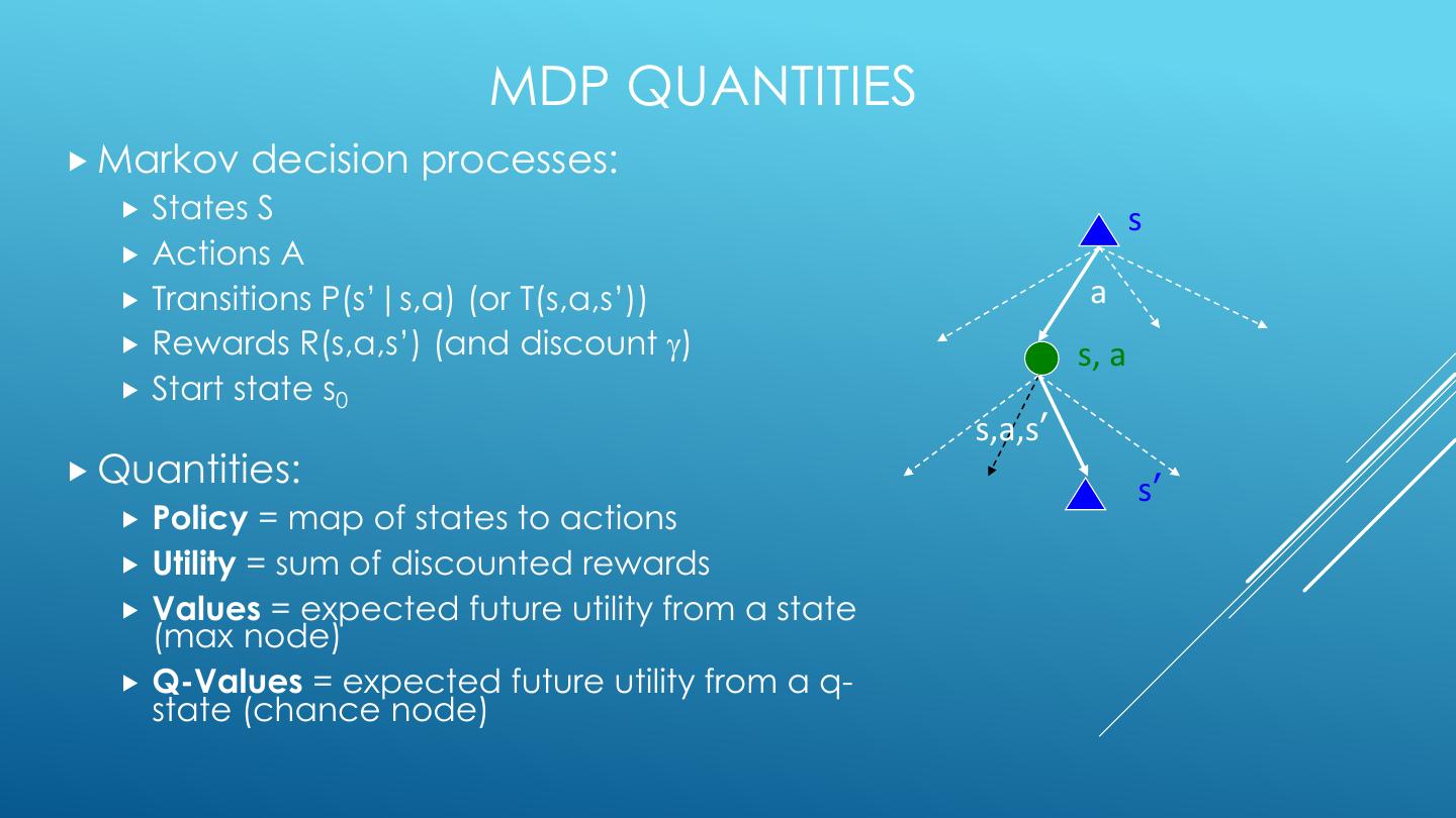
15 . MDP QUANTITIES  Markov decision processes:  States S s  Actions A  Transitions P(s’|s,a) (or T(s,a,s’)) a  Rewards R(s,a,s’) (and discount ) s, a  Start state s0 s,a,s’  Quantities: s’  Policy = map of states to actions  Utility = sum of discounted rewards  Values = expected future utility from a state (max node)  Q-Values = expected future utility from a q- state (chance node) 

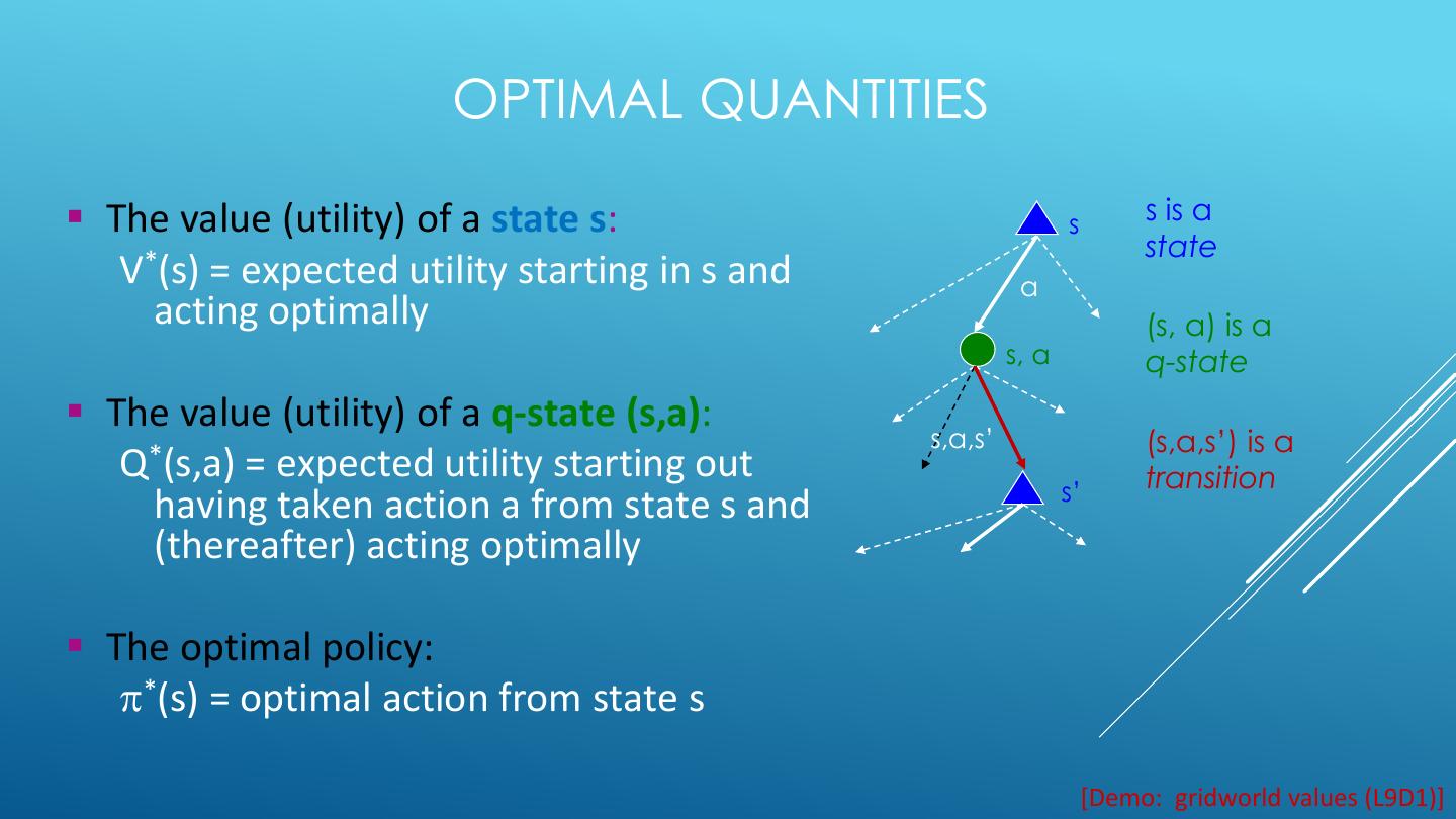
16 . OPTIMAL QUANTITIES ▪ The value (utility) of a state s: s s is a state V*(s) = expected utility starting in s and a acting optimally (s, a) is a s, a q-state ▪ The value (utility) of a q-state (s,a): s,a,s’ (s,a,s’) is a Q*(s,a) = expected utility starting out transition s’ having taken action a from state s and (thereafter) acting optimally ▪ The optimal policy: *(s) = optimal action from state s [Demo: gridworld values (L9D1)] 

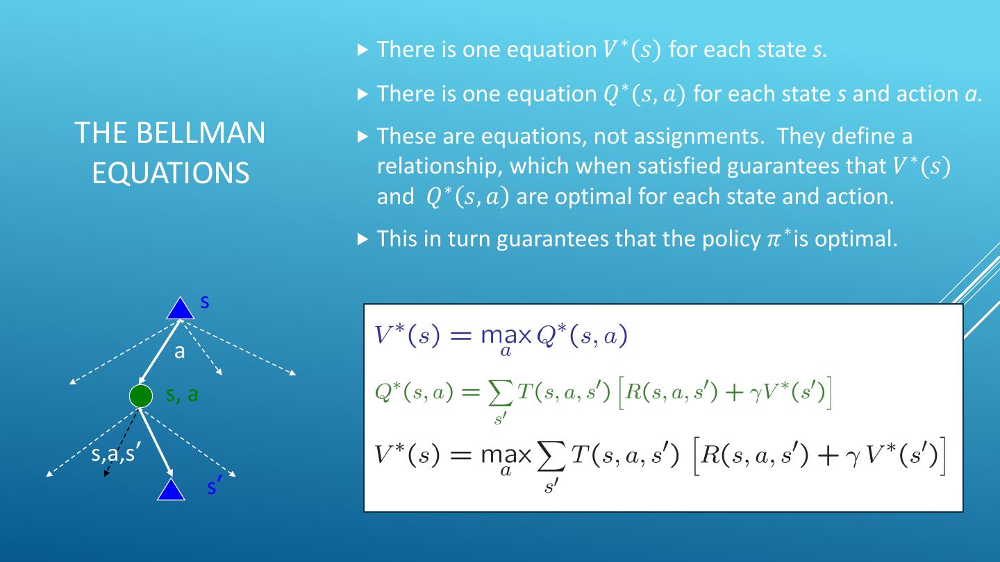
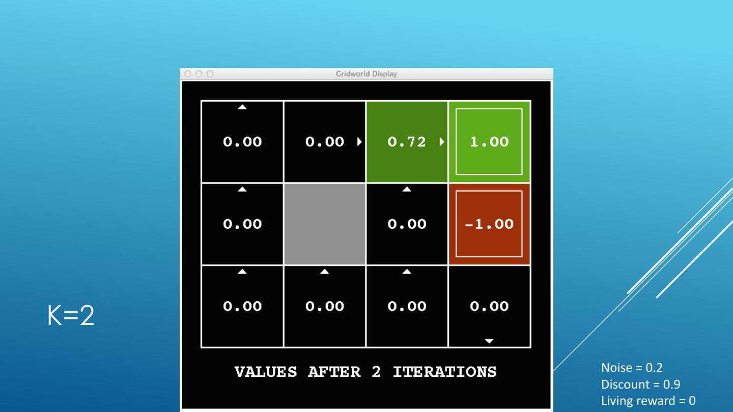
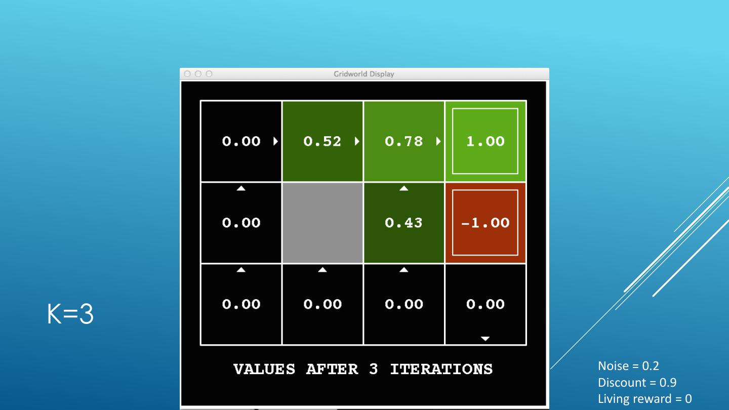
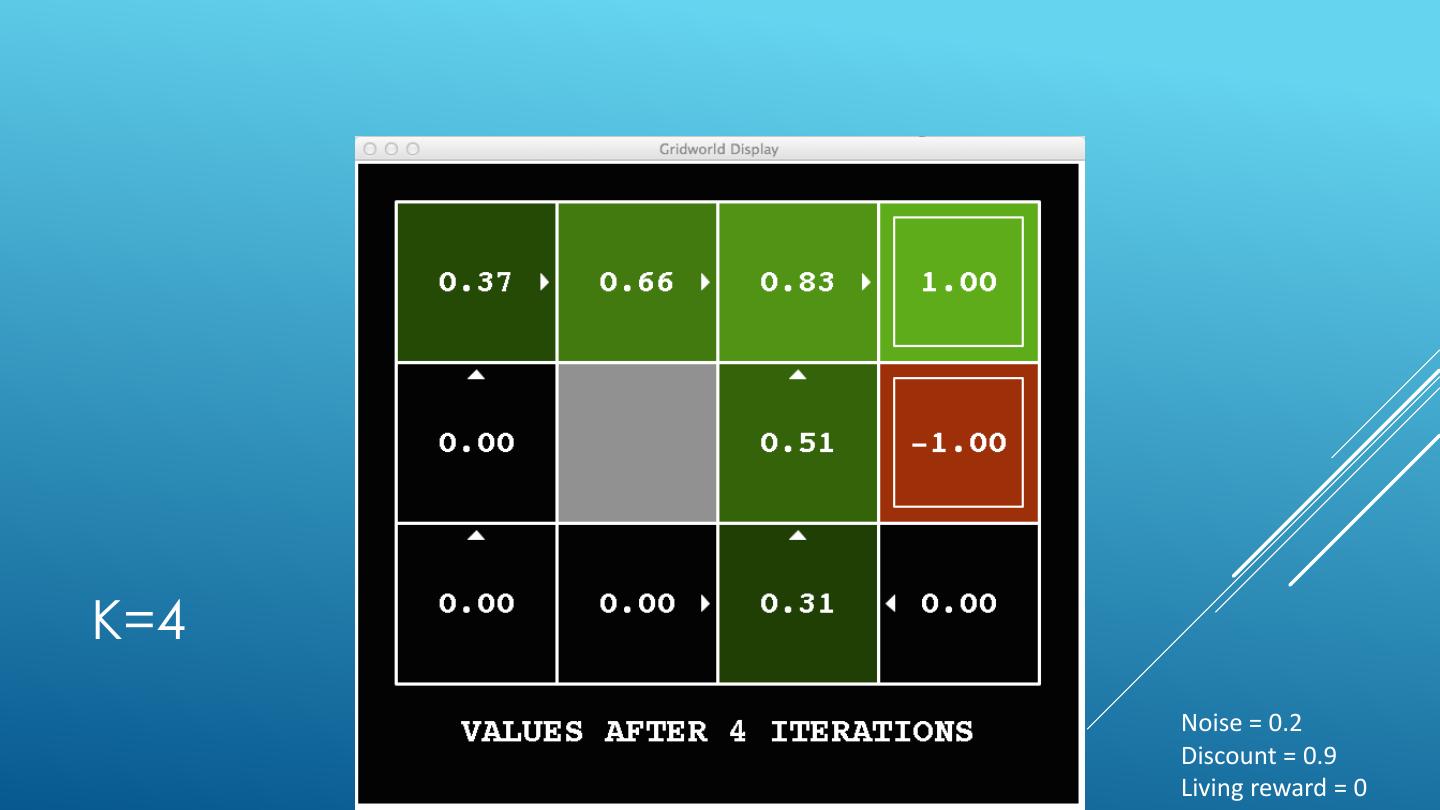
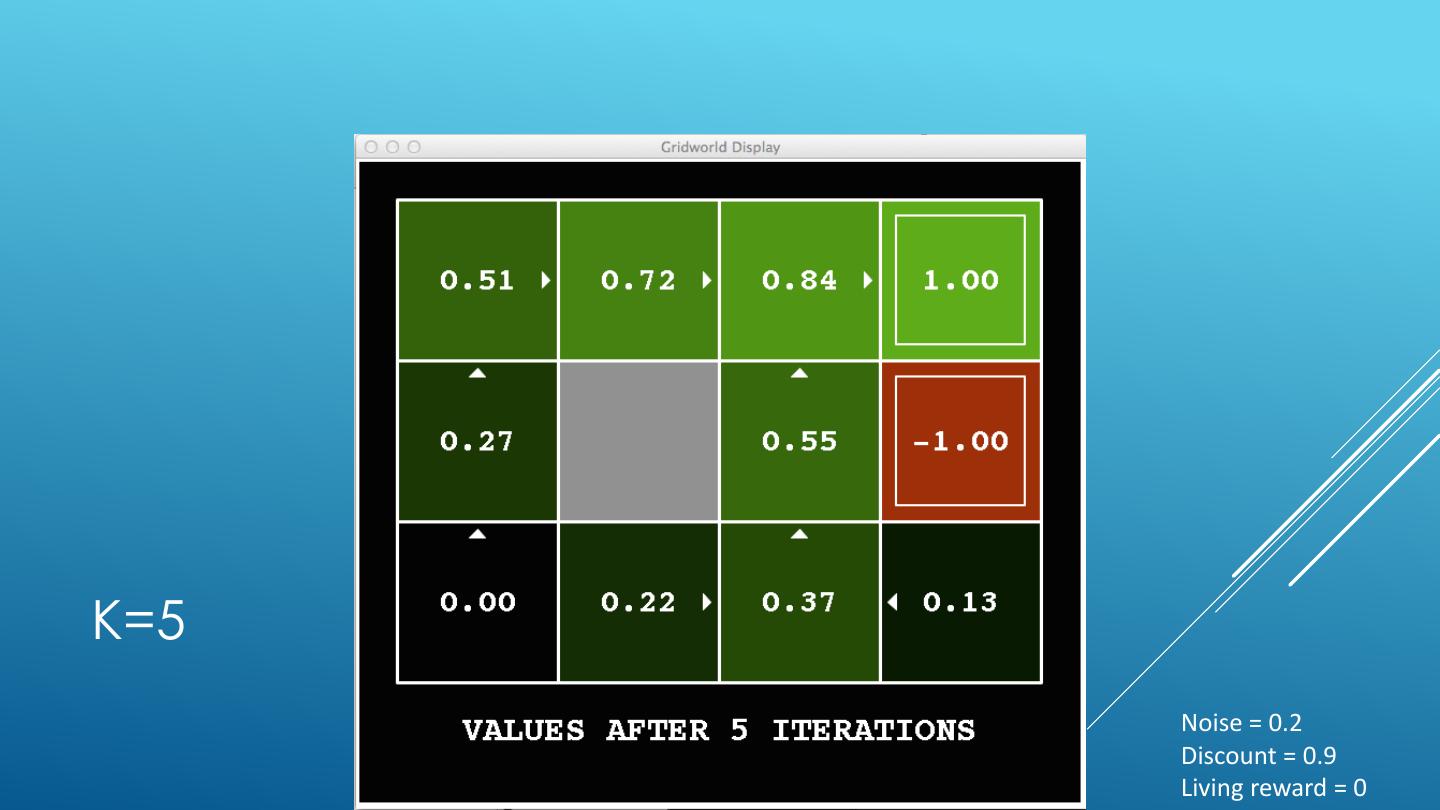
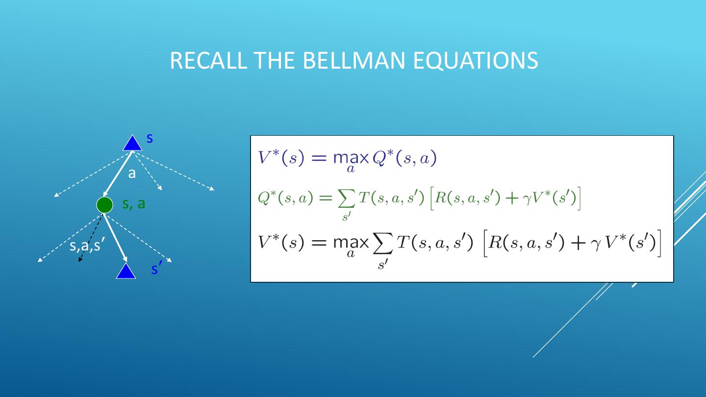
17 .  There is one equation 𝑉 ∗ (𝑠) for each state s.  There is one equation 𝑄 ∗ (𝑠, 𝑎) for each state s and action a. THE BELLMAN  These are equations, not assignments. They define a EQUATIONS relationship, which when satisfied guarantees that 𝑉 ∗ (𝑠) and 𝑄 ∗ 𝑠, 𝑎 are optimal for each state and action.  This in turn guarantees that the policy 𝜋 ∗ is optimal. s a s, a s,a,s’ s’ 

18 .4 MDP ALGORITHMS 

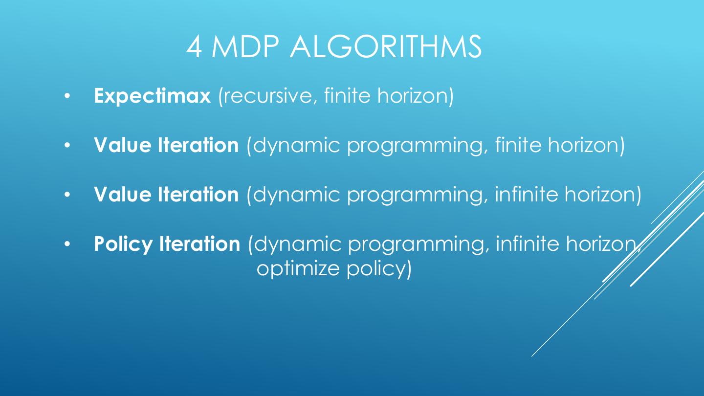
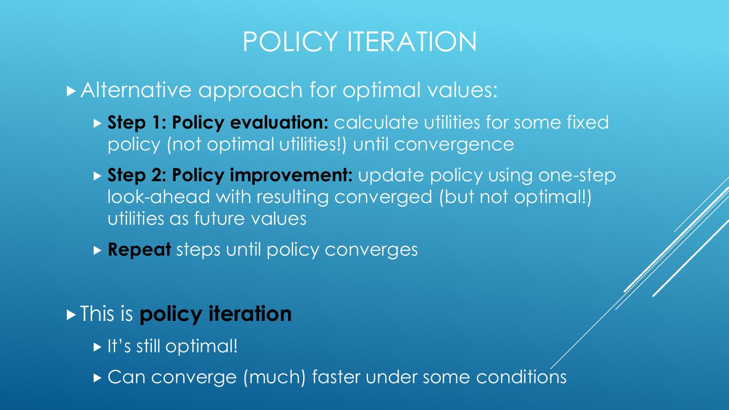
19 . 4 MDP ALGORITHMS • Expectimax (recursive, finite horizon) • Value Iteration (dynamic programming, finite horizon) • Value Iteration (dynamic programming, infinite horizon) • Policy Iteration (dynamic programming, infinite horizon, optimize policy) 

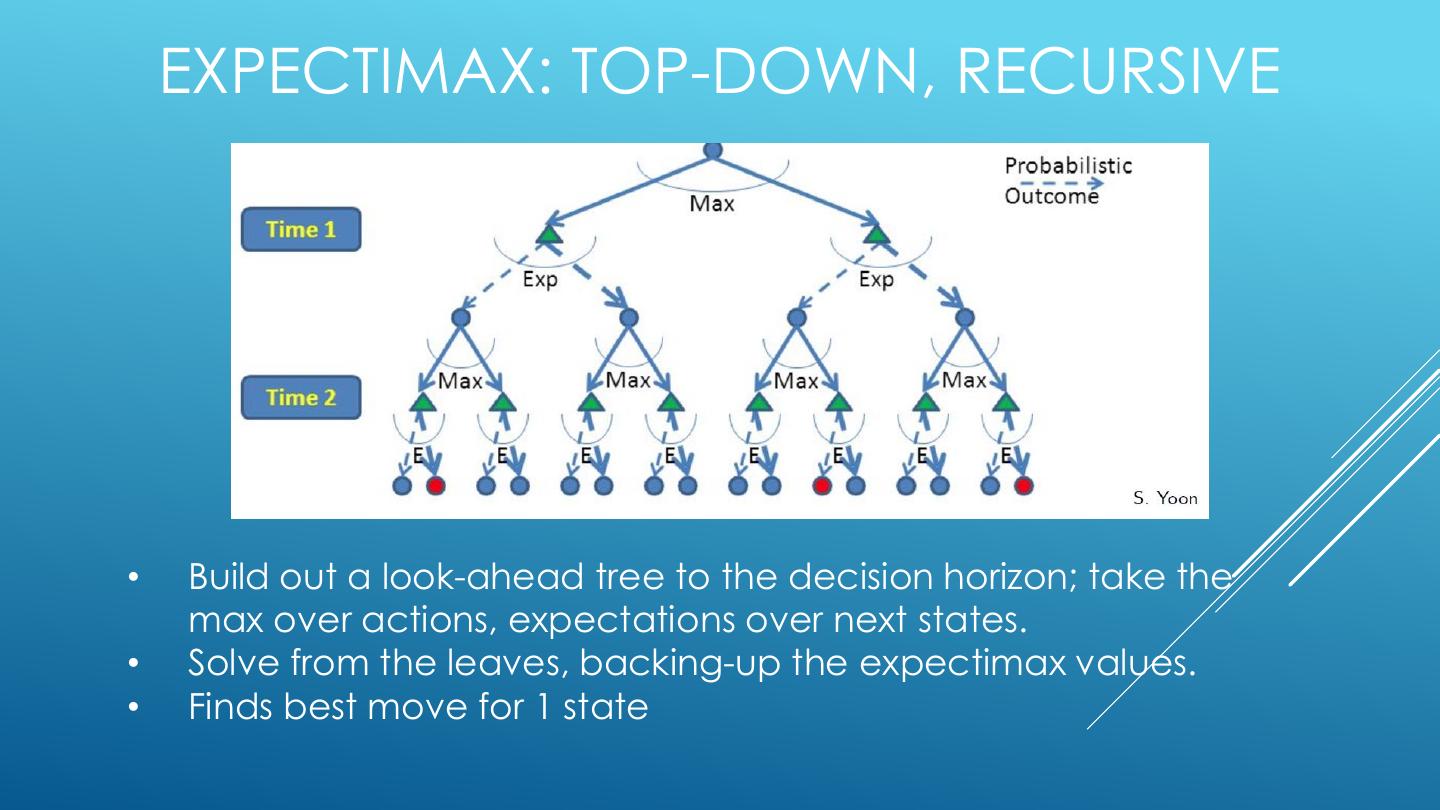
20 . EXPECTIMAX: TOP-DOWN, RECURSIVE • Build out a look-ahead tree to the decision horizon; take the max over actions, expectations over next states. • Solve from the leaves, backing-up the expectimax values. • Finds best move for 1 state 

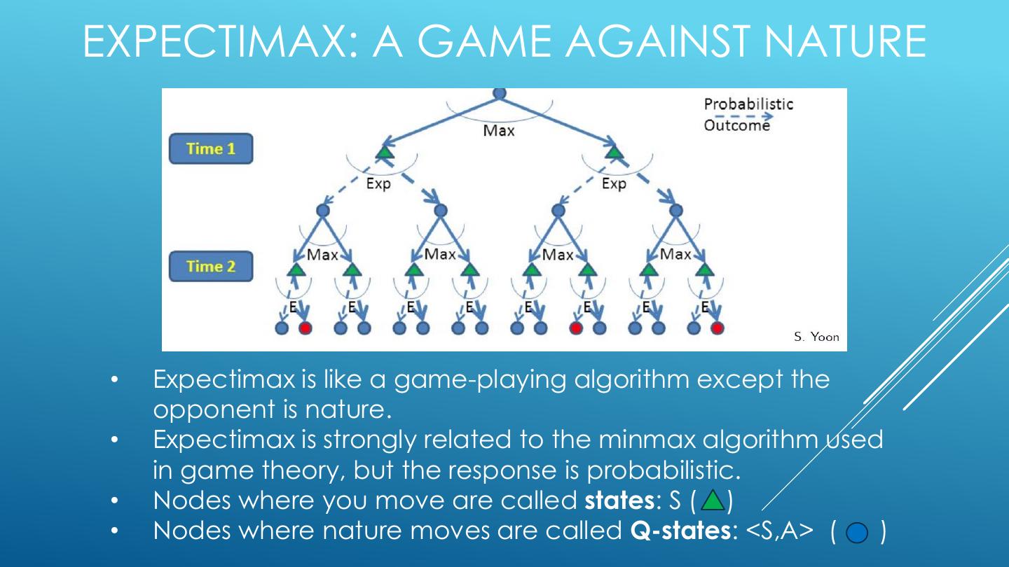
21 .EXPECTIMAX: A GAME AGAINST NATURE • Expectimax is like a game-playing algorithm except the opponent is nature. • Expectimax is strongly related to the minmax algorithm used in game theory, but the response is probabilistic. • Nodes where you move are called states: S ( ) • Nodes where nature moves are called Q-states: <S,A> ( ) 

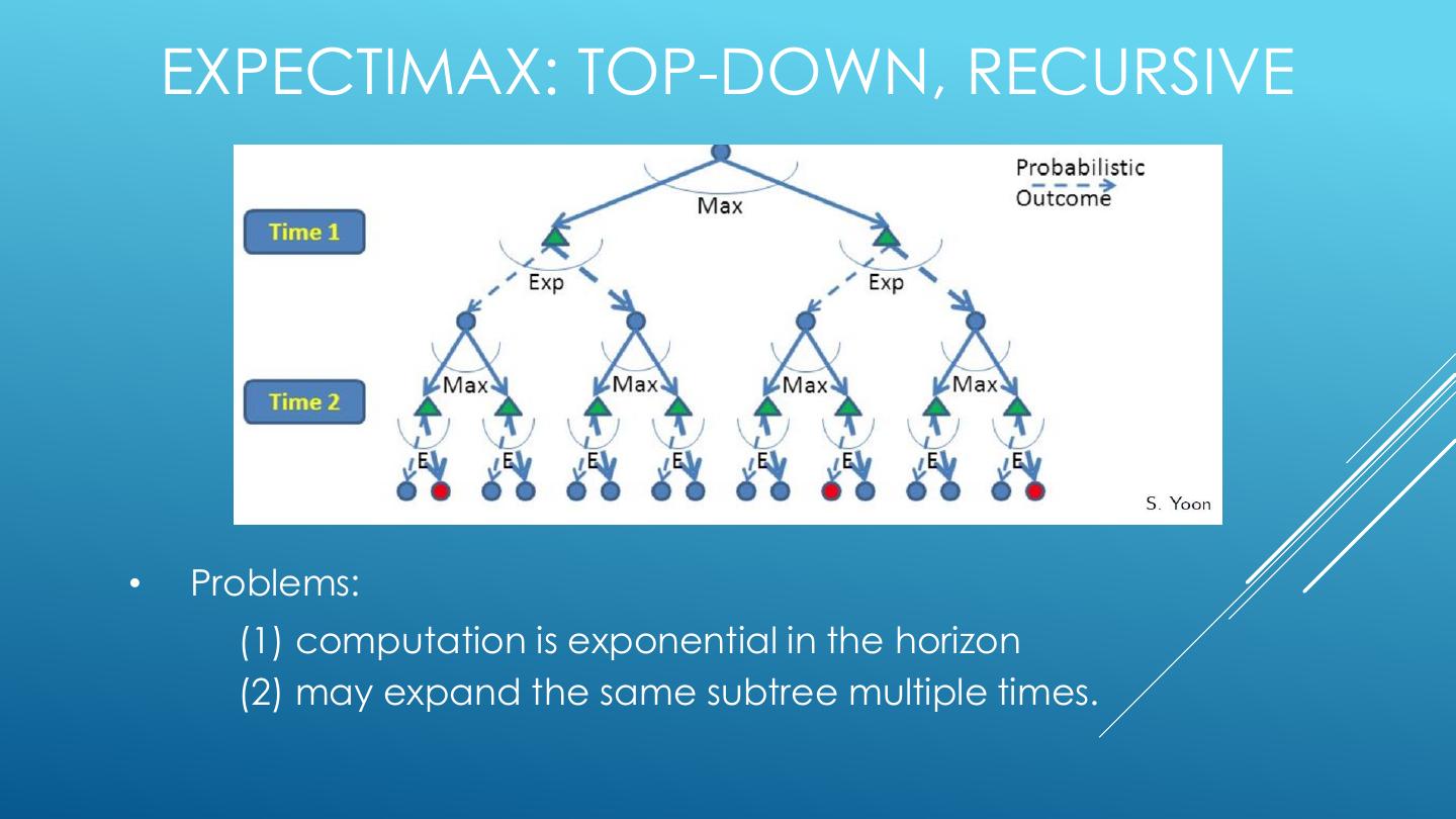
22 . EXPECTIMAX: TOP-DOWN, RECURSIVE • Problems: (1) computation is exponential in the horizon (2) may expand the same subtree multiple times. 

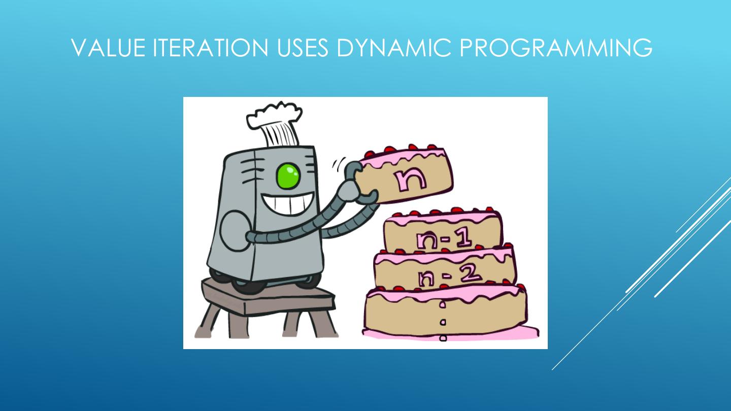
23 .VALUE ITERATION USES DYNAMIC PROGRAMMING 

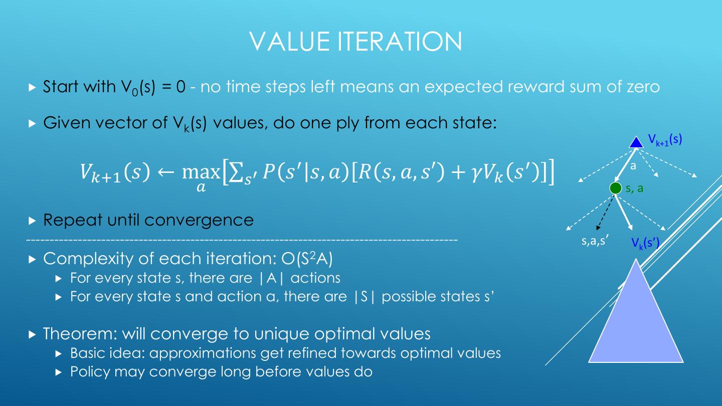
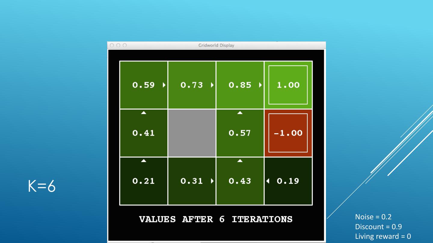
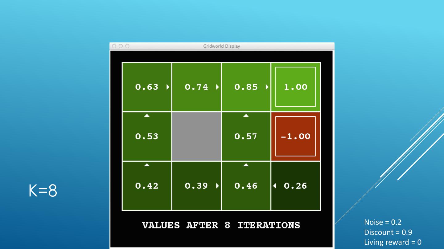
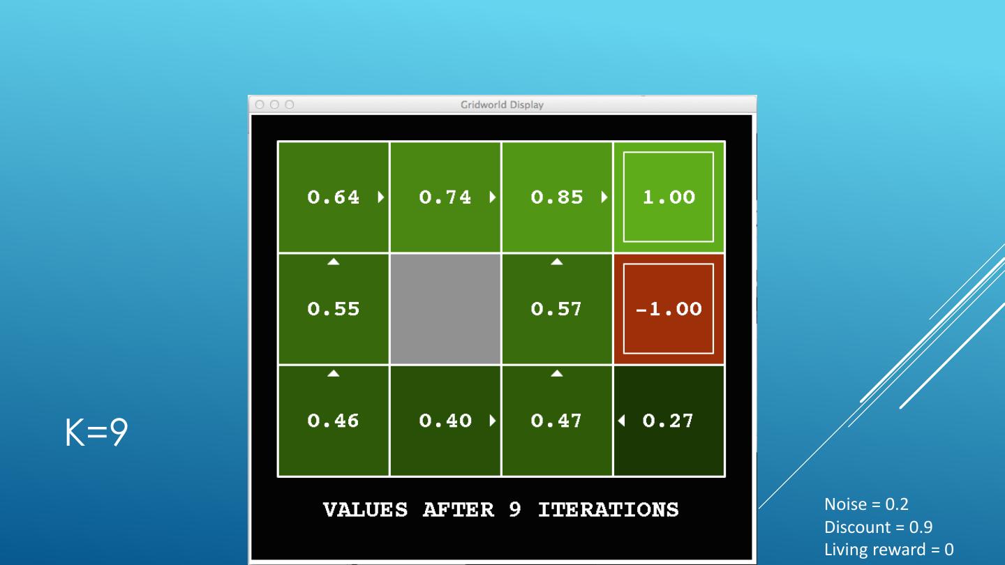
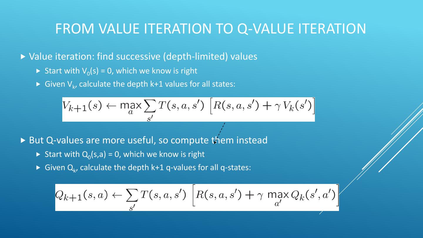
24 . VALUE ITERATION  Start with V0(s) = 0 - no time steps left means an expected reward sum of zero  Given vector of Vk(s) values, do one ply from each state: Vk+1(s) 𝑉𝑘+1 𝑠 ← max σ𝑠′ 𝑃 𝑠 ′ 𝑠, 𝑎 𝑅 𝑠, 𝑎, 𝑠′ + 𝛾𝑉𝑘 𝑠 ′ a 𝑎 s, a  Repeat until convergence -------------------------------------------------------------------------------------------- s,a,s’ Vk(s’)  Complexity of each iteration: O(S2A)  For every state s, there are |A| actions  For every state s and action a, there are |S| possible states s’  Theorem: will converge to unique optimal values  Basic idea: approximations get refined towards optimal values  Policy may converge long before values do 

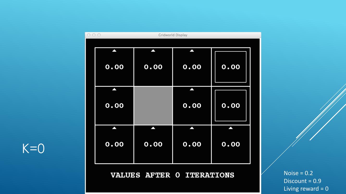
25 .K=0 Noise = 0.2 Discount = 0.9 Living reward = 0 

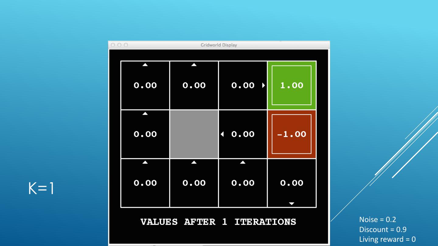
26 .K=1 Noise = 0.2 Discount = 0.9 Living reward = 0 

27 .K=2 Noise = 0.2 Discount = 0.9 Living reward = 0 

28 .K=3 Noise = 0.2 Discount = 0.9 Living reward = 0 

29 .K=4 Noise = 0.2 Discount = 0.9 Living reward = 0