Regularization

1 .Regularization Attempt to prevent overfitting Gene Olafsen

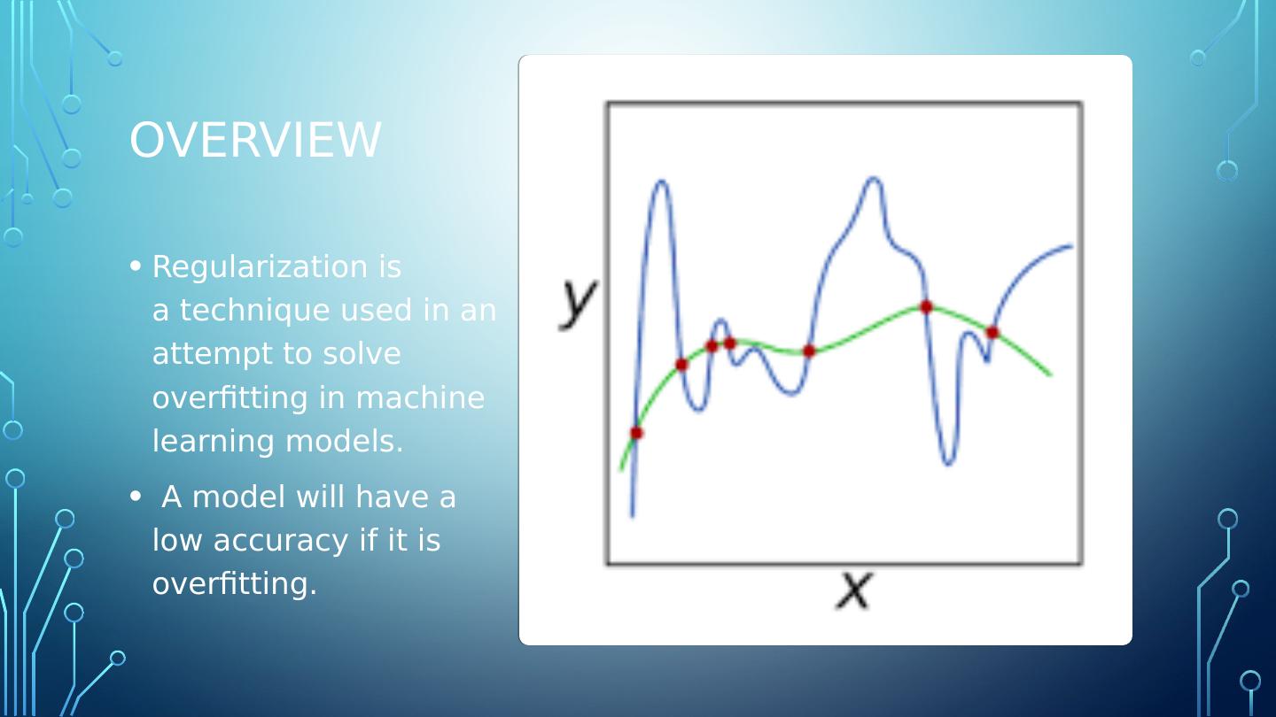
2 .overview Regularization is a technique used in an attempt to solve overfitting in machine learning models.  A model will have a low accuracy if it is overfitting.

3 .why Typically, a model is trying too hard and capturing noise in the training dataset, or the data points that don’t really represent the true properties of the data. Learning such data points, makes the model more flexible, at the risk of overfitting. Summary: A well trained model is low on bias and variance.

4 .validation Validation: The process of deciding whether the numerical results quantifying hypothesized relationships between variables, are acceptable as descriptions of the data. Types of Validation: Holdout Method K-Fold Cross Validation Starfield K-Fold Cross Validation Leave-one-out Validation Leave-P-Out Cross Validation

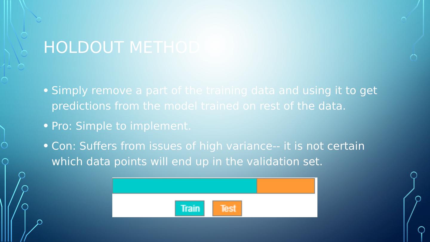
5 .Holdout Method Simply remove a part of the training data and using it to get predictions from the model trained on rest of the data. Pro: Simple to implement. Con: Suffers from issues of high variance-- it is not certain which data points will end up in the validation set.

6 .Removing Data for Validation Holding out data for validation can be problematic. Removing a part of the data for validation poses a problem of the model underfitting. By reducing the training data, there is a risk of losing important patterns/ trends in data set, which in turn increases error induced by bias.

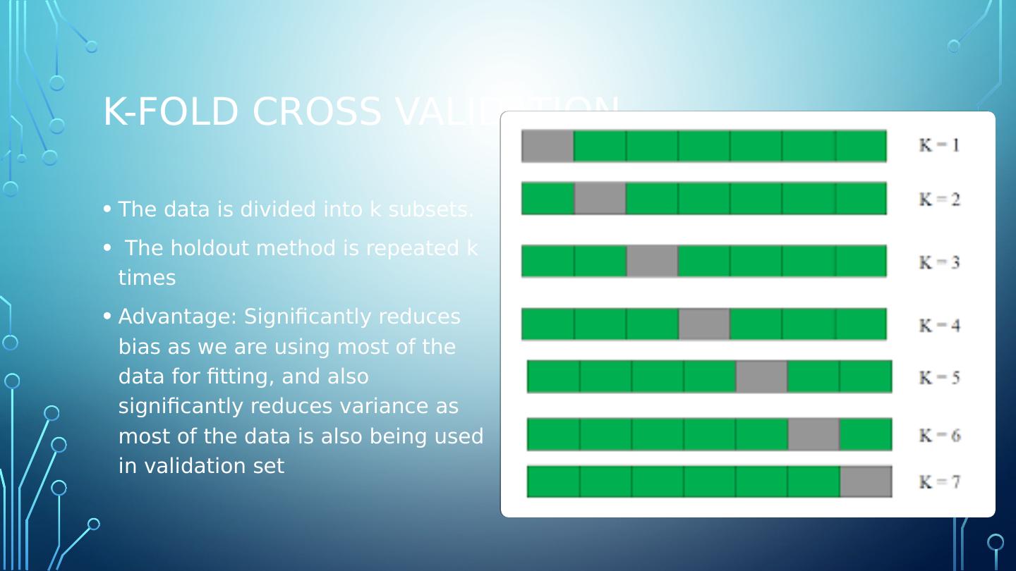
7 .K-Fold Cross Validation The data is divided into k subsets.  The holdout method is repeated k times Advantage: Significantly reduces bias as we are using most of the data for fitting, and also significantly reduces variance as most of the data is also being used in validation set

8 .Starfield K-Fold Cross Validation In some cases, there may be a large imbalance in the response variables. In dataset concerning price of houses, there might be large number of houses having high price. In case of classification, there might be several times more negative samples than positive samples.

9 .Starfield Course correction Simply modify the typical K-fold cross validation sample such that each fold contains approximately the same percentage of samples of each target class as the complete set. In the case of prediction problems, correct the samples such that the mean response value is approximately equal in all of the folds.

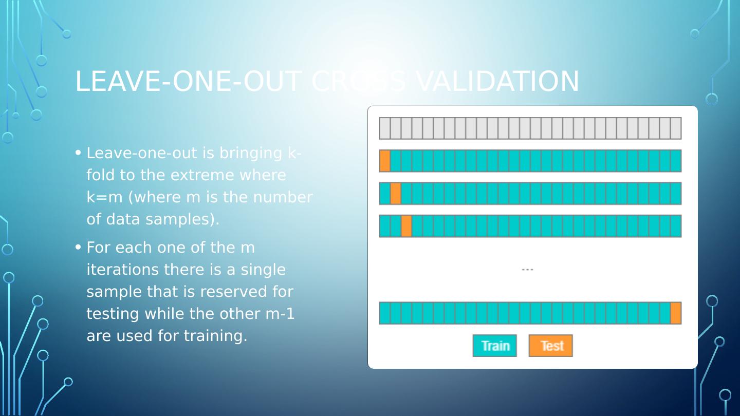
10 .Leave-one-out cross validation Leave-one-out is bringing k-fold to the extreme where k=m (where m is the number of data samples). For each one of the m iterations there is a single sample that is reserved for testing while the other m-1 are used for training.

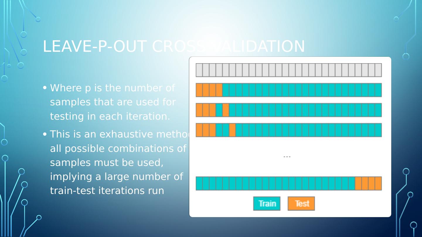
11 .Leave-P-Out Cross Validation Where p is the number of samples that are used for testing in each iteration. This is an exhaustive method, all possible combinations of p samples must be used, implying a large number of train-test iterations run

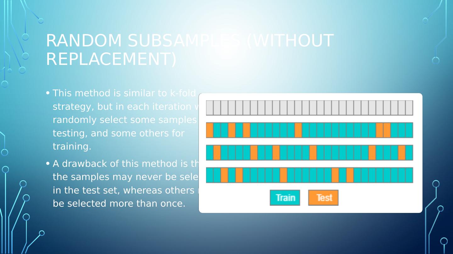
12 .Random subsamples (without replacement) This method is similar to k-fold strategy, but in each iteration we randomly select some samples for testing, and some others for training. A drawback of this method is that the samples may never be selected in the test set, whereas others may be selected more than once.

13 .Early stopping To avoid overfitting the training set- one solution is just to stop training.  In practice, this can be accomplished by saving a model snapshot at regular intervals and then comparing the current training against the previous snapshot. If performance starts dropping- simply restore the previous model. Note: Higher performance can generally be achieved by combining early stopping with other regularization techniques.

14 .LaSso and ridge regularization  A tuning parameter is added which lets you change the complexity or smoothness of the model. The regularization value imposes a special penalty on complex models.

15 .L1 - LASSO LASSO (least absolute shrinkage and selection operator) L1 is the sum of the weights. adds “absolute value of magnitude” of coefficient as penalty term to the loss function a lot of non-zero coefficients When to use:  Lasso shrinks the less important feature’s coefficient to zero thus, removing some feature altogether. This works well for feature selection in cases having a huge number of features.

16 .L2 - Ridge Ridge Regression L2 is the sum of the square of the weights. models with large coefficients adds “squared magnitude” of coefficient as penalty term to the loss function

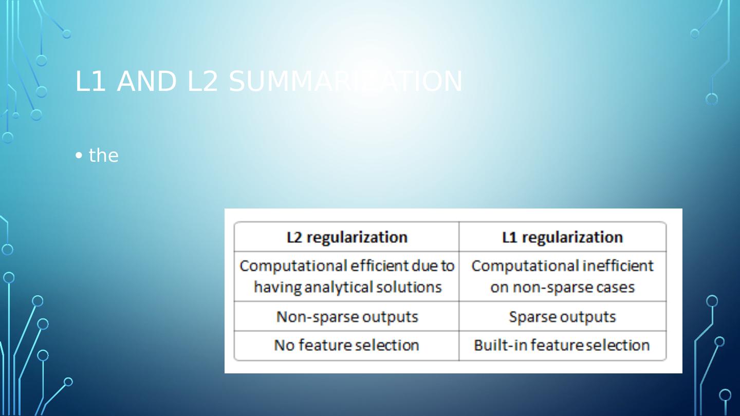
17 .L1 and L2 Summarization the

18 .dropout Proposed by G.E. Hinton in 2012 and further refined by Nitish Srivastava. State-of-the-art neural networks receive a 1-2% boost in accuracy by utilizing dropout. For 95% accurate models this means dropping the error rate by almost 40%. 

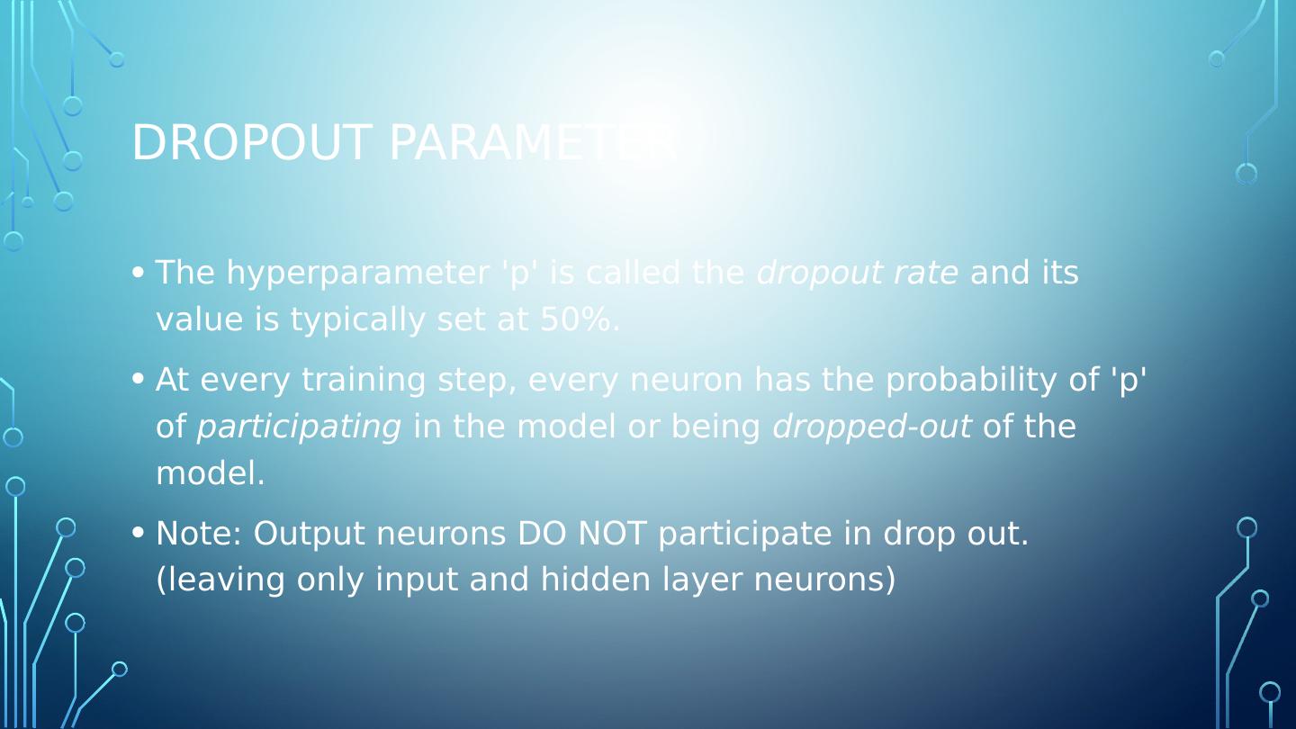
19 .Dropout parameter The hyperparameter p is called the dropout rate  and its value is typically set at 50%. At every training step, every neuron has the probability of p of participating  in the model or being dropped-out of the model. Note: Output neurons DO NOT participate in drop out. (leaving only input and hidden layer neurons)

20 .Dropout for real

21 .Why does dropout work? The resulting neural network can be seen as an averaging ensemble of the smaller neural networks produced during the training steps.

22 .Using a model trained with dropout You need to multiply each neurons input connection weights by the dropout p value after training. So if the model was trained with 50% dropout, the input connection weights must be multiplied by 0.5 after training. If you dont... each neuron will get a total input signal roughly twice as large as what the network was trained on.

23 .Max-norm regularization Constrains the weights w, clipping w if it exceeds hyperparameter r after each training step. Reducing r increases the amount of regularization and helps reduce overfitting. TensorFlow does not implement Max-Norm Regularization. It is not difficult to implement. The machine learning book provides an example. Keras provides Max-Norm regularization out of the box.

24 .Data augmentation Generating new training instances from existing data to boost the size of the training set. Common transformations include image shift, rotate, resize and contrast. Note: Adding white noise does not augment data because white noise is not learnable.

25 .Default deep neural network configuration Initialization: He initialization Activation Function: ELU Normalization: Batch Normalization Regularization: Dropout Optimizer Nesterov Accelerated Gradient Learning Rate Schedule: None

26 .Regularization guidelines If convergence is too slow, then try a learning schedule that utilizes exponential decay. If the training set is too small, try implementing data augmentation. To achieve a sparse model, add l1 (LASSO) regularization- and zero out tiny weights after training. To achieve an even sparser model, try FTRL instead of Adam optization along with l1 regularization. For a fast runtime model, do not use Batch Normalization and replace ELU activation function with leaky ReLU . (Also a sparse model helps) From: Hands-on Machine Learning with Scikit -Learn & TensorFlow