Model-based RL

1 .MODEL-BASED REINFORCEMENT LEARNING 

2 . The material for this talk is drawn from the slides, notes and lectures from several offerings of the CS181 course at Harvard University:  CS181 Intelligent Machines: Perception, Learning and Uncertainty, Sarah Finney, Spring 2009  CS181 Intelligent Machines: Perception, Learning and Uncertainty, Prof. David C Brooks, Spring 2011 CS181 – Machine Learning, Prof. Ryan P. Adams, Spring REFERENCES  2014. https://github.com/wihl/cs181-spring2014  CS181 – Machine Learning, Prof. David Parkes, Spring 2017. https://harvard-ml-courses.github.io/cs181-web- 2017/ As well as notes and lectures from Stanford course CS229 :  CS229 – Machine Learning, Andrew Ng. https://see.stanford.edu/Course/CS229 

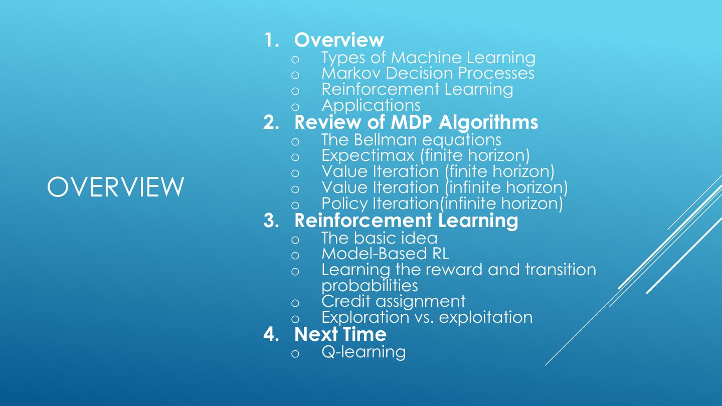
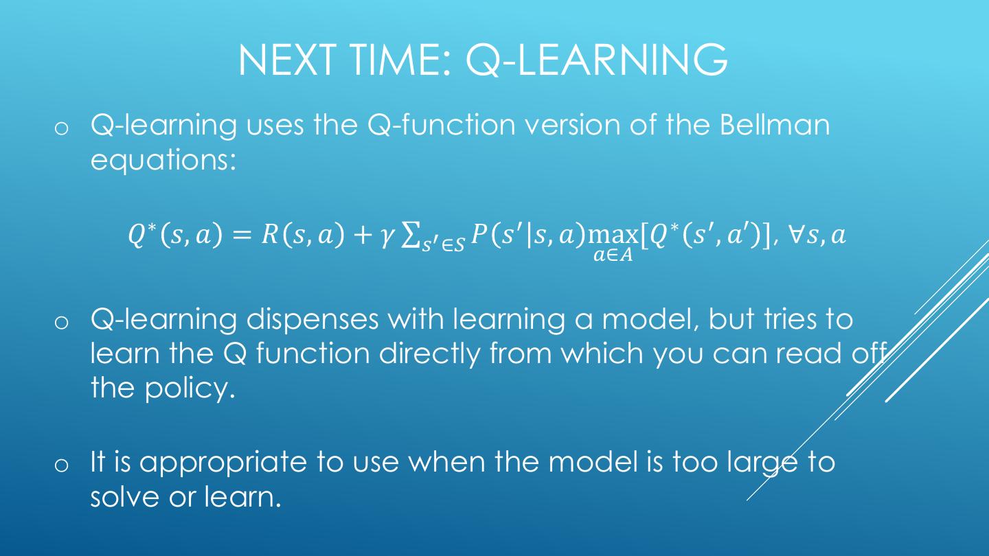
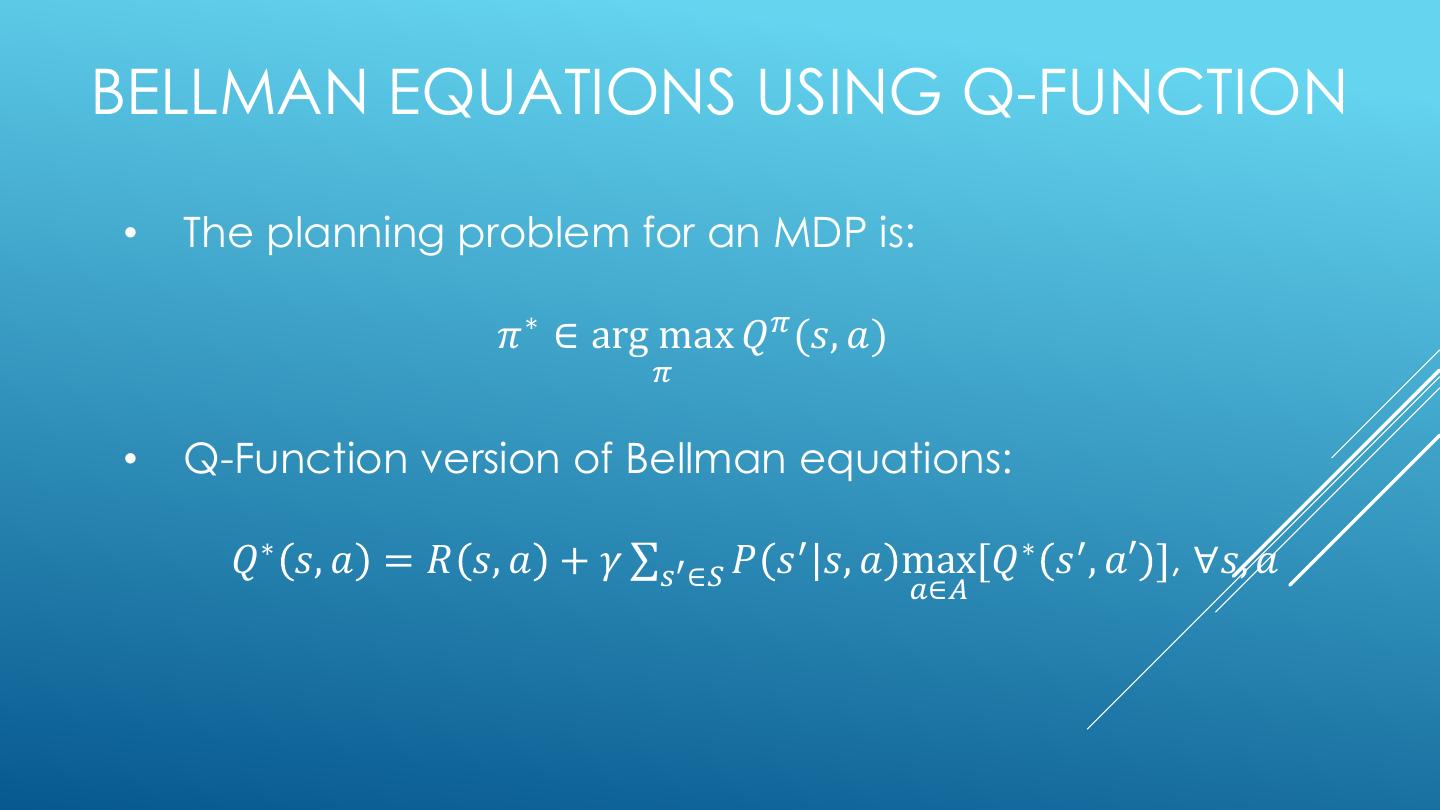
3 . 1. Overview o Types of Machine Learning o Markov Decision Processes o Reinforcement Learning o Applications 2. Review of MDP Algorithms o The Bellman equations o Expectimax (finite horizon) o Value Iteration (finite horizon) OVERVIEW o o Value Iteration (infinite horizon) Policy Iteration(infinite horizon) 3. Reinforcement Learning o The basic idea o Model-Based RL o Learning the reward and transition probabilities o Credit assignment o Exploration vs. exploitation 4. Next Time o Q-learning 

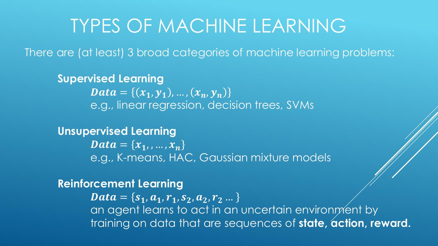
4 . TYPES OF MACHINE LEARNING There are (at least) 3 broad categories of machine learning problems: Supervised Learning 𝑫𝒂𝒕𝒂 = 𝒙𝟏 , 𝒚𝟏 , … , 𝒙𝒏 , 𝒚𝒏 e.g., linear regression, decision trees, SVMs Unsupervised Learning 𝑫𝒂𝒕𝒂 = 𝒙𝟏 , , … , 𝒙𝒏 e.g., K-means, HAC, Gaussian mixture models Reinforcement Learning 𝑫𝒂𝒕𝒂 = 𝒔𝟏 , 𝒂𝟏 , 𝒓𝟏 , 𝒔𝟐 , 𝒂𝟐 , 𝒓𝟐 … an agent learns to act in an uncertain environment by training on data that are sequences of state, action, reward. 

5 . MARKOV DECISION PROCESSES • Markov Decision Processes provide a mathematical framework for modeling decision making in situations where outcomes are partly random and partly under the control of a decision maker. • The initial analysis of MDPs assume complete knowledge of states, actions, rewards, transitions, and discounts. <https://en.wikipedia.org/w/index.php?title=Markov_decision_process&oldid=855934986> [accessed 11 September 2018] 

6 . MARKOV DECISION PROCESSES • States: 𝒔𝟏 , … , 𝒔𝒏 • Actions: 𝒂𝟏 , … , 𝒂𝒎 • Reward Function: r 𝑠, 𝑎 ∈ 𝑅 • Transition model: p 𝑠′ 𝑠, 𝑎 • Discount factor: γ ∈ 𝟎, 𝟏 <https://en.wikipedia.org/w/index.php?title=Markov_decision_process&oldid=855934986> [accessed 11 September 2018] 

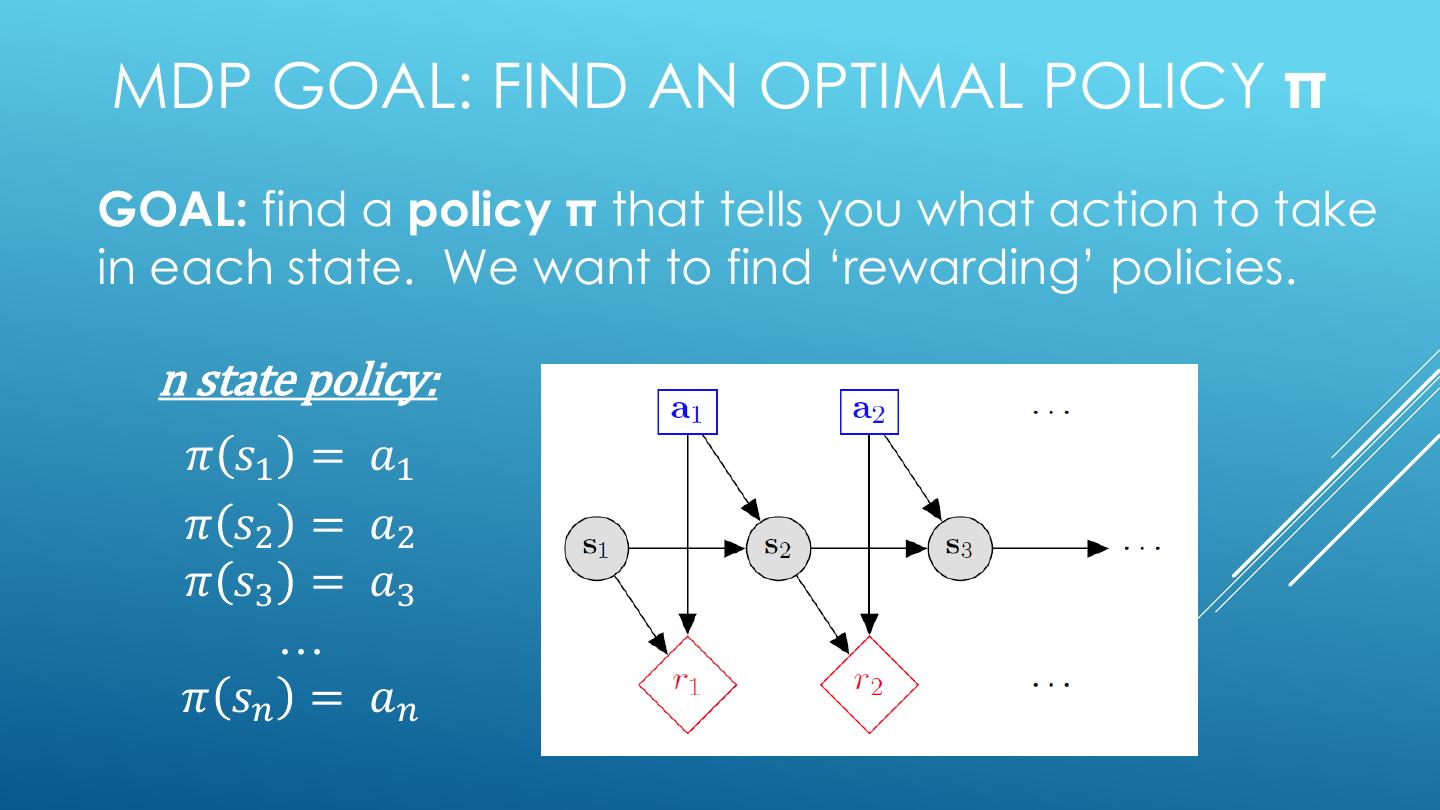
7 .MDP GOAL: FIND AN OPTIMAL POLICY π GOAL: find a policy π that tells you what action to take in each state. We want to find ‘rewarding’ policies. n state policy: 𝜋 𝑠1 = 𝑎1 𝜋 𝑠2 = 𝑎2 𝜋 𝑠3 = 𝑎3 … 𝜋 𝑠𝑛 = 𝑎𝑛 

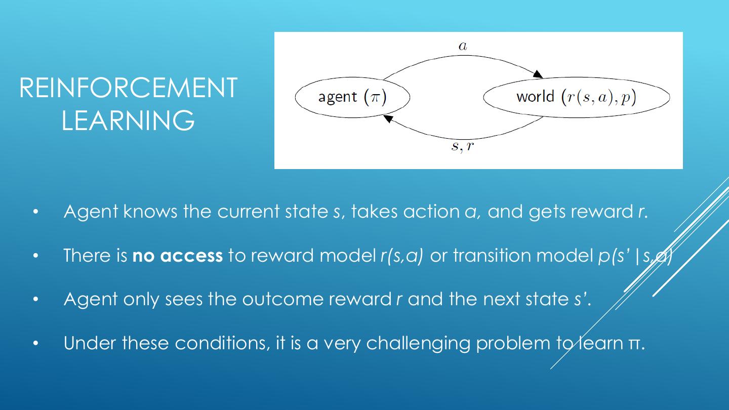
8 .REINFORCEMENT LEARNING • Agent knows the current state s, takes action a, and gets reward r. • There is no access to reward model r(s,a) or transition model p(s’|s,a) • Agent only sees the outcome reward r and the next state s’. • Under these conditions, it is a very challenging problem to learn π. 

9 .REVIEW OF MDP ALGORITHMS 

10 . REVIEW OF MDP ALGORITHMS There are 4 standard MDP algorithms that assume complete knowledge: • Expectimax (finite horizon, 𝛾 = 1) • Value Iteration (finite horizon, 𝛾 = 1) • Value Iteration (infinite horizon, 𝛾 ∈ [0,1)) • Policy Iteration (infinite horizon , 𝛾 ∈ [0,1)) 

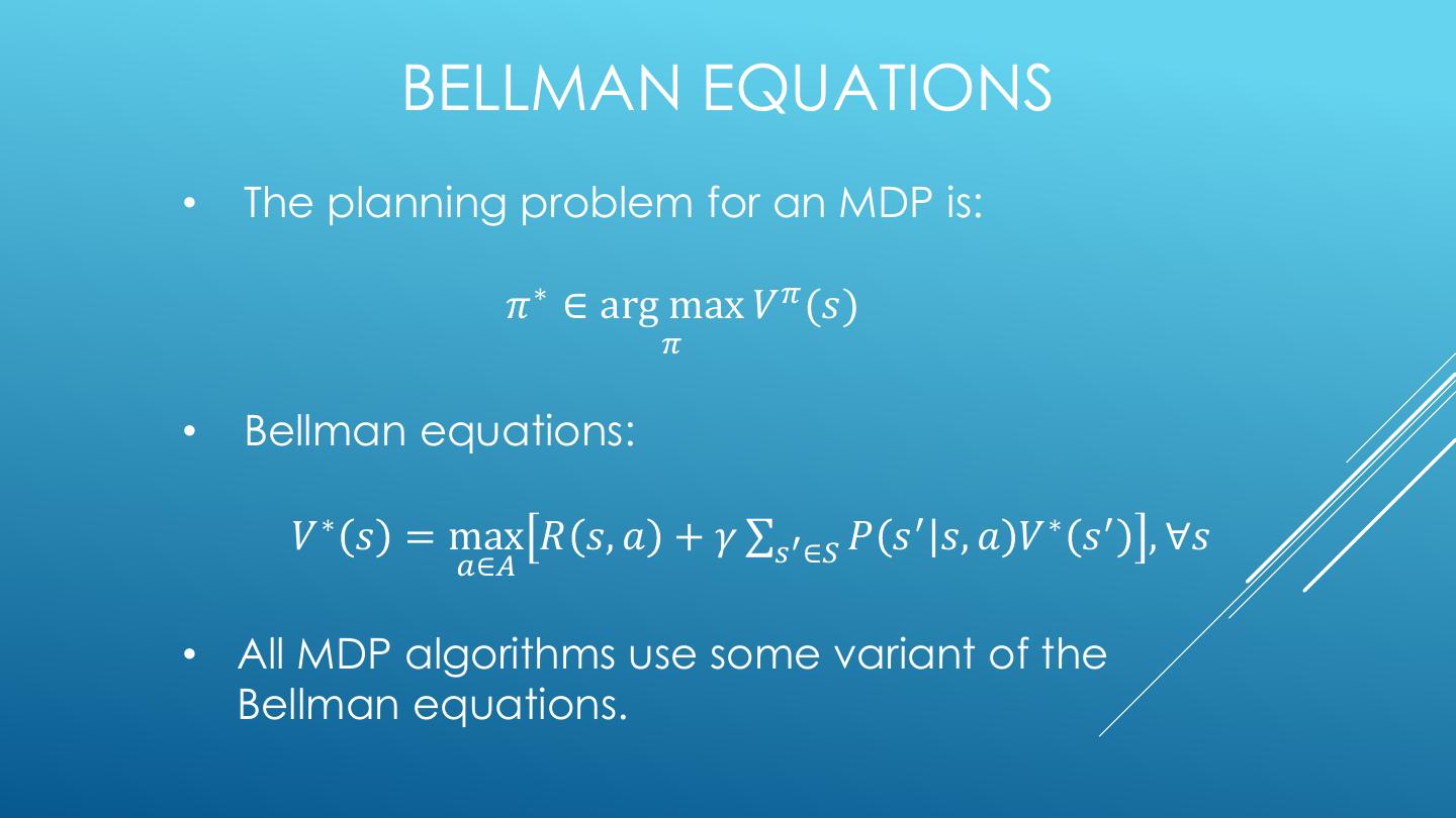
11 . BELLMAN EQUATIONS • The planning problem for an MDP is: 𝜋 ∗ ∈ arg max 𝑉 𝜋 (𝑠) 𝜋 • Bellman equations: 𝑉 ∗ 𝑠 = max 𝑅 𝑠, 𝑎 + 𝛾 σ𝑠′ ∈𝑆 𝑃 𝑠 ′ 𝑠, 𝑎 𝑉 ∗ 𝑠 ′ , ∀𝑠 𝑎∈𝐴 • All MDP algorithms use some variant of the Bellman equations. 

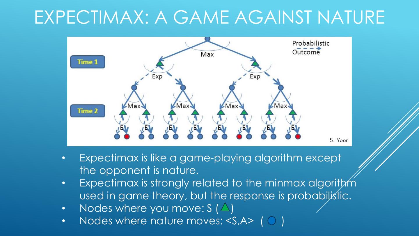
12 . EXPECTIMAX: TOP-DOWN, RECURSIVE • Build out a look-ahead tree to the decision horizon; take the max over actions, expectations over next states. • Solve from the leaves, backing-up the expectimax values. • Problems: (1) computation is exponential in the horizon; (2) may expand the same subtree multiple times. 

13 .EXPECTIMAX: A GAME AGAINST NATURE • Expectimax is like a game-playing algorithm except the opponent is nature. • Expectimax is strongly related to the minmax algorithm used in game theory, but the response is probabilistic. • Nodes where you move: S ( ) • Nodes where nature moves: <S,A> ( ) 

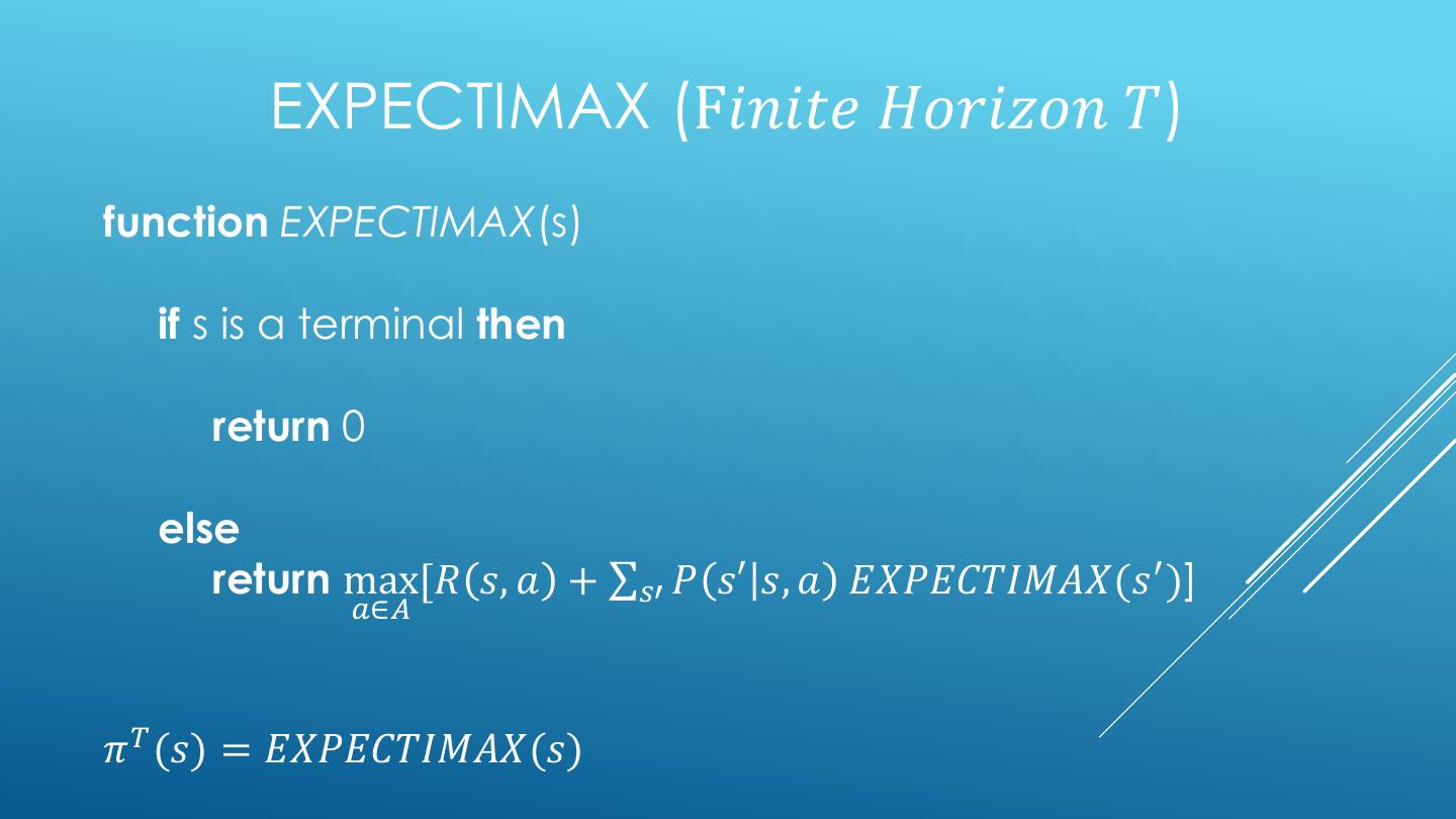
14 . EXPECTIMAX (F𝑖𝑛𝑖𝑡𝑒 𝐻𝑜𝑟𝑖𝑧𝑜𝑛 𝑇) function EXPECTIMAX(s) if s is a terminal then return 0 else return max[𝑅 𝑠, 𝑎 + σ𝑠′ 𝑃 𝑠′ 𝑠, 𝑎 𝐸𝑋𝑃𝐸𝐶𝑇𝐼𝑀𝐴𝑋(𝑠 ′ )] 𝑎∈𝐴 𝜋 𝑇 (𝑠) = 𝐸𝑋𝑃𝐸𝐶𝑇𝐼𝑀𝐴𝑋(𝑠) 

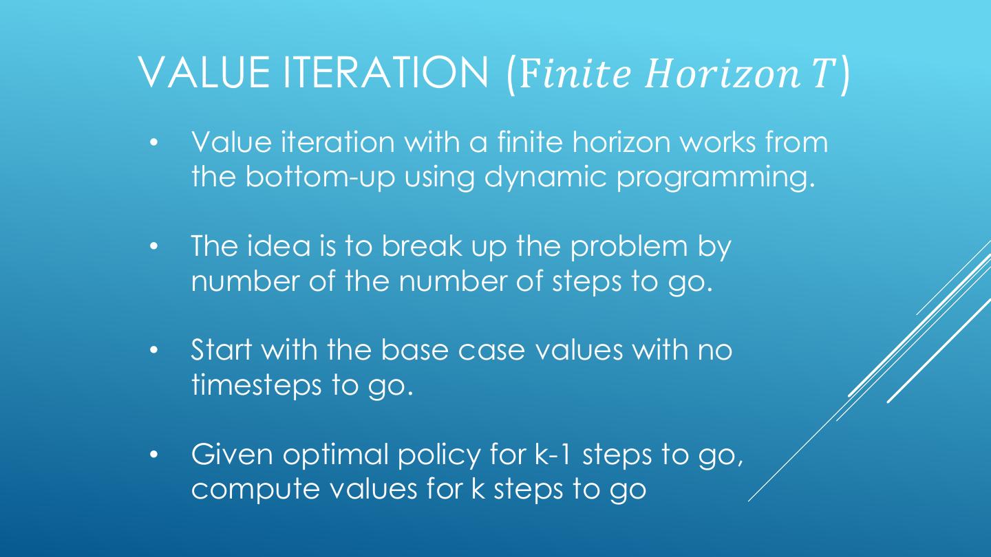
15 .VALUE ITERATION (F𝑖𝑛𝑖𝑡𝑒 𝐻𝑜𝑟𝑖𝑧𝑜𝑛 𝑇) • Value iteration with a finite horizon works from the bottom-up using dynamic programming. • The idea is to break up the problem by number of the number of steps to go. • Start with the base case values with no timesteps to go. • Given optimal policy for k-1 steps to go, compute values for k steps to go 

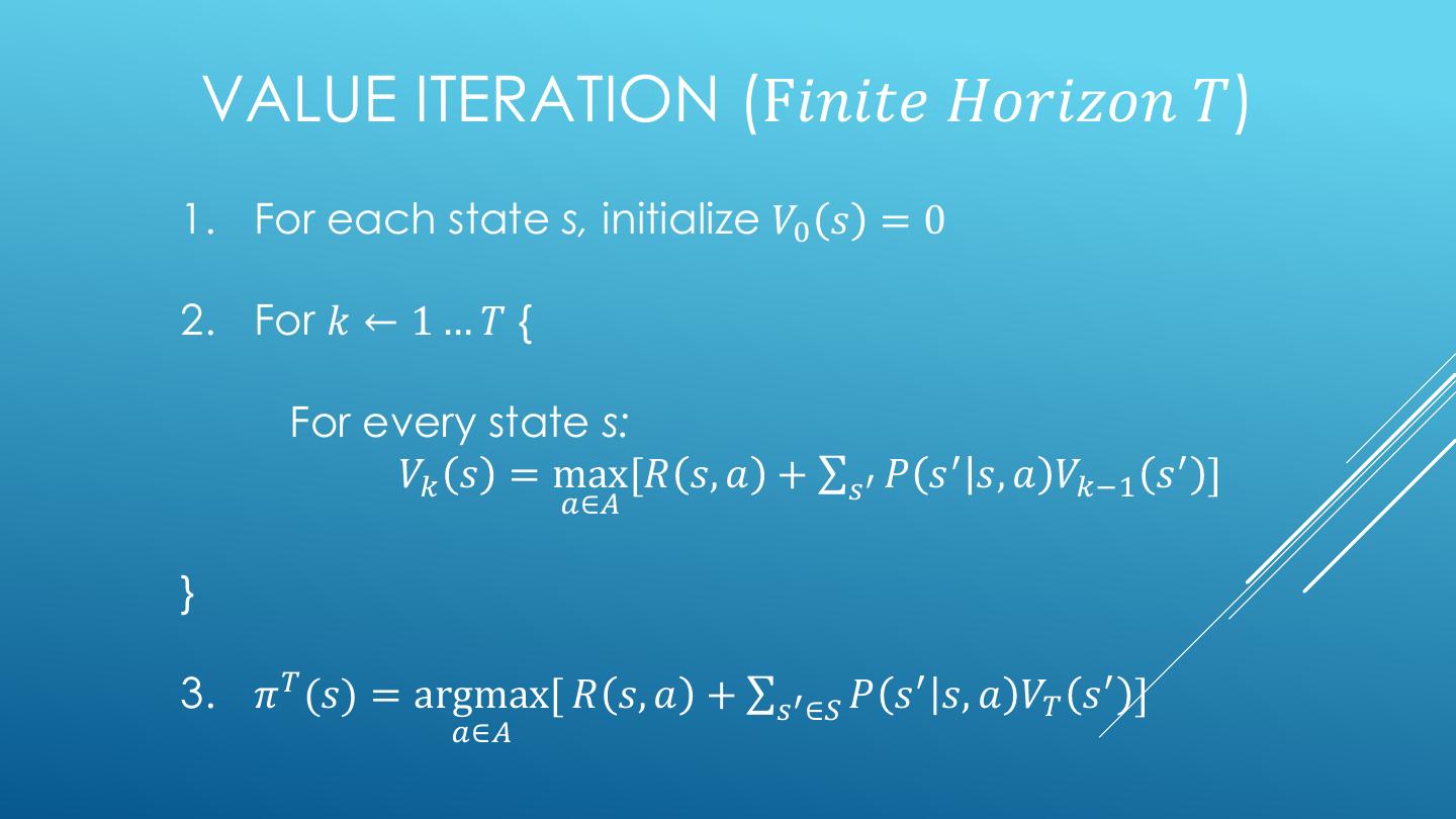
16 . VALUE ITERATION (F𝑖𝑛𝑖𝑡𝑒 𝐻𝑜𝑟𝑖𝑧𝑜𝑛 𝑇) 1. For each state s, initialize 𝑉0 𝑠 = 0 2. For 𝑘 ← 1 … 𝑇 { For every state s: 𝑉𝑘 𝑠 = max[𝑅 𝑠, 𝑎 + σ𝑠′ 𝑃 𝑠 ′ 𝑠, 𝑎 𝑉𝑘−1 𝑠 ′ ] 𝑎∈𝐴 } 3. 𝜋 𝑇 (𝑠) = argmax[ 𝑅 𝑠, 𝑎 + σ𝑠′ ∈𝑆 𝑃 𝑠 ′ 𝑠, 𝑎 𝑉𝑇 𝑠 ′ ] 𝑎∈𝐴 

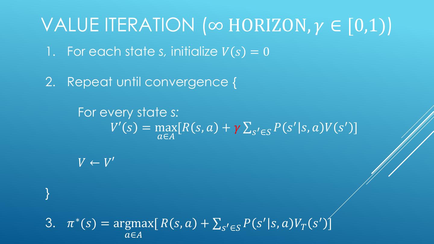
17 .VALUE ITERATION (∞ HORIZON, 𝛾 ∈ [0,1)) • Value iteration with an infinite horizon is a generalization of value iteration with a finite horizon. • The main change is that the discount factor 𝛾 is set to less than one discounting the value of states farther in the future. • It can be shown that 𝑉 will converge over time to 𝑉 ∗ • Iterate the update equation until the changes in 𝑉 fall below some 𝜖. 

18 .VALUE ITERATION (∞ HORIZON, 𝛾 ∈ [0,1)) 1. For each state s, initialize 𝑉 𝑠 = 0 2. Repeat until convergence { For every state s: 𝑉′ 𝑠 = max[𝑅 𝑠, 𝑎 + 𝛾 σ𝑠′ ∈𝑆 𝑃 𝑠 ′ 𝑠, 𝑎 𝑉 𝑠 ′ ] 𝑎∈𝐴 𝑉 ← 𝑉′ } 3. 𝜋 ∗ (𝑠) = argmax[ 𝑅 𝑠, 𝑎 + σ𝑠′ ∈𝑆 𝑃 𝑠 ′ 𝑠, 𝑎 𝑉𝑇 𝑠 ′ ] 𝑎∈𝐴 

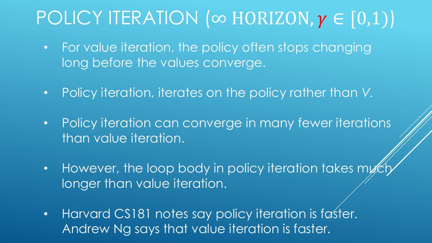
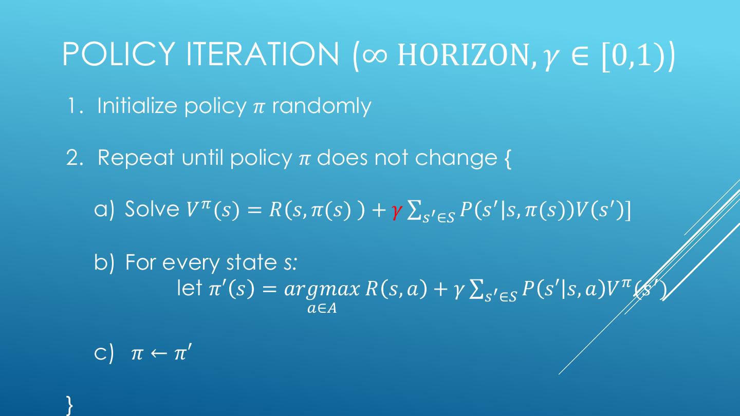
19 .POLICY ITERATION (∞ HORIZON, 𝛾 ∈ [0,1)) • For value iteration, the policy often stops changing long before the values converge. • Policy iteration, iterates on the policy rather than V. • Policy iteration can converge in many fewer iterations than value iteration. • However, the loop body in policy iteration takes much longer than value iteration. • Harvard CS181 notes say policy iteration is faster. Andrew Ng says that value iteration is faster. 

20 .POLICY ITERATION (∞ HORIZON, 𝛾 ∈ [0,1)) 1. Initialize policy 𝜋 randomly 2. Repeat until policy 𝜋 does not change { a) Solve 𝑉 𝜋 (𝑠) = 𝑅 𝑠, 𝜋(𝑠) + 𝛾 σ𝑠′ ∈𝑆 𝑃 𝑠 ′ 𝑠, 𝜋(𝑠) 𝑉 𝑠 ′ ] b) For every state s: let 𝜋′ 𝑠 = 𝑎𝑟𝑔𝑚𝑎𝑥 𝑅 𝑠, 𝑎 + 𝛾 σ𝑠′ ∈𝑆 𝑃 𝑠′ 𝑠, 𝑎 𝑉 𝜋 (𝑠 ′ ) 𝑎∈𝐴 c) 𝜋 ← 𝜋′ } 

21 .REINFORCEMENT LEARNING 

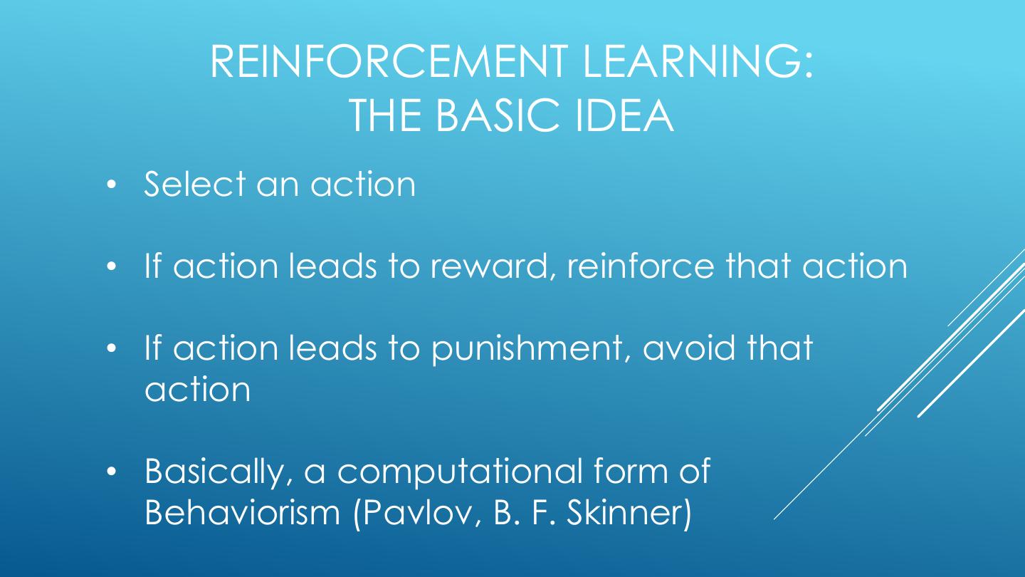
22 . REINFORCEMENT LEARNING: THE BASIC IDEA • Select an action • If action leads to reward, reinforce that action • If action leads to punishment, avoid that action • Basically, a computational form of Behaviorism (Pavlov, B. F. Skinner) 

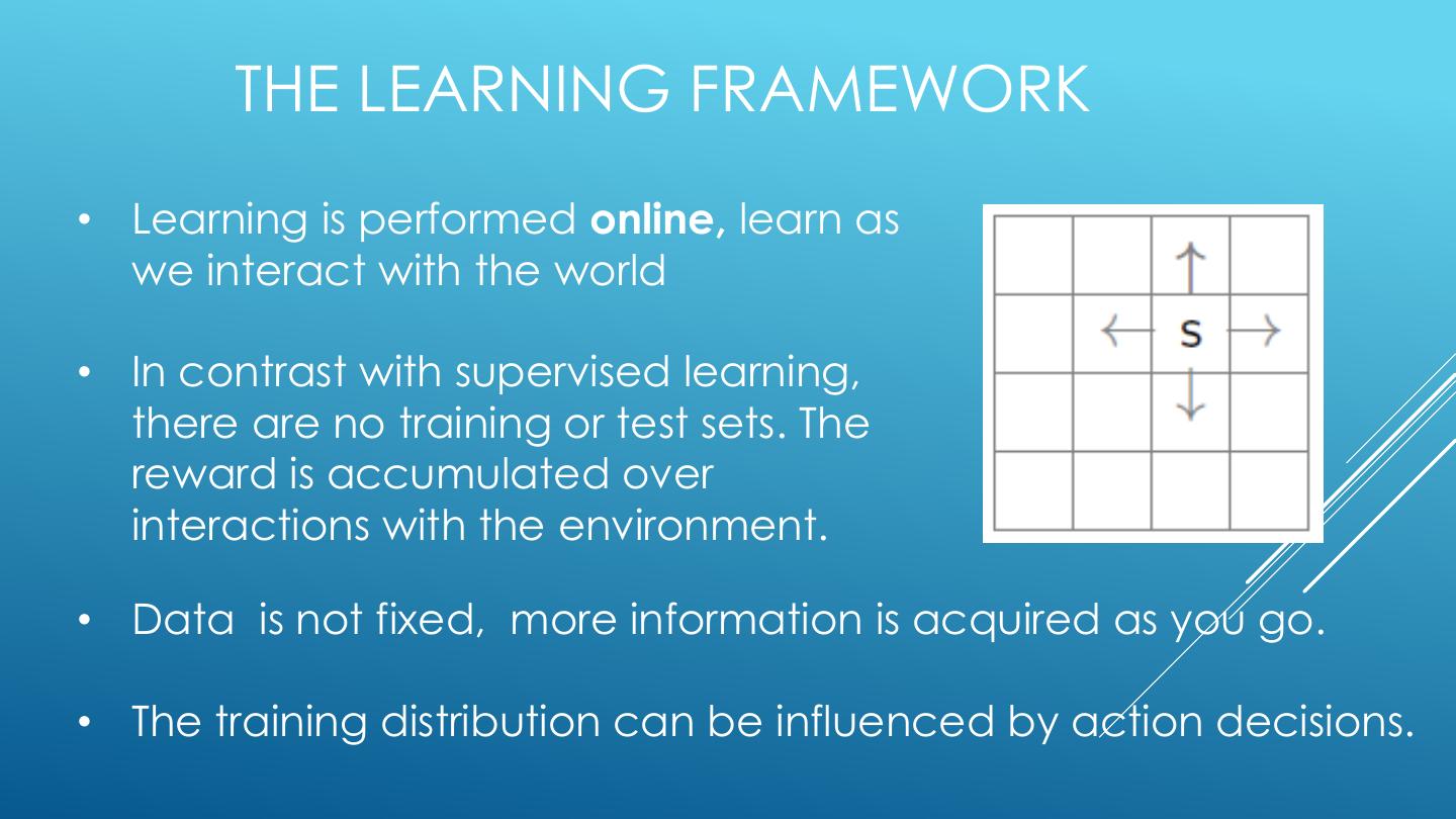
23 . THE LEARNING FRAMEWORK • Learning is performed online, learn as we interact with the world • In contrast with supervised learning, there are no training or test sets. The reward is accumulated over interactions with the environment. • Data is not fixed, more information is acquired as you go. • The training distribution can be influenced by action decisions. 

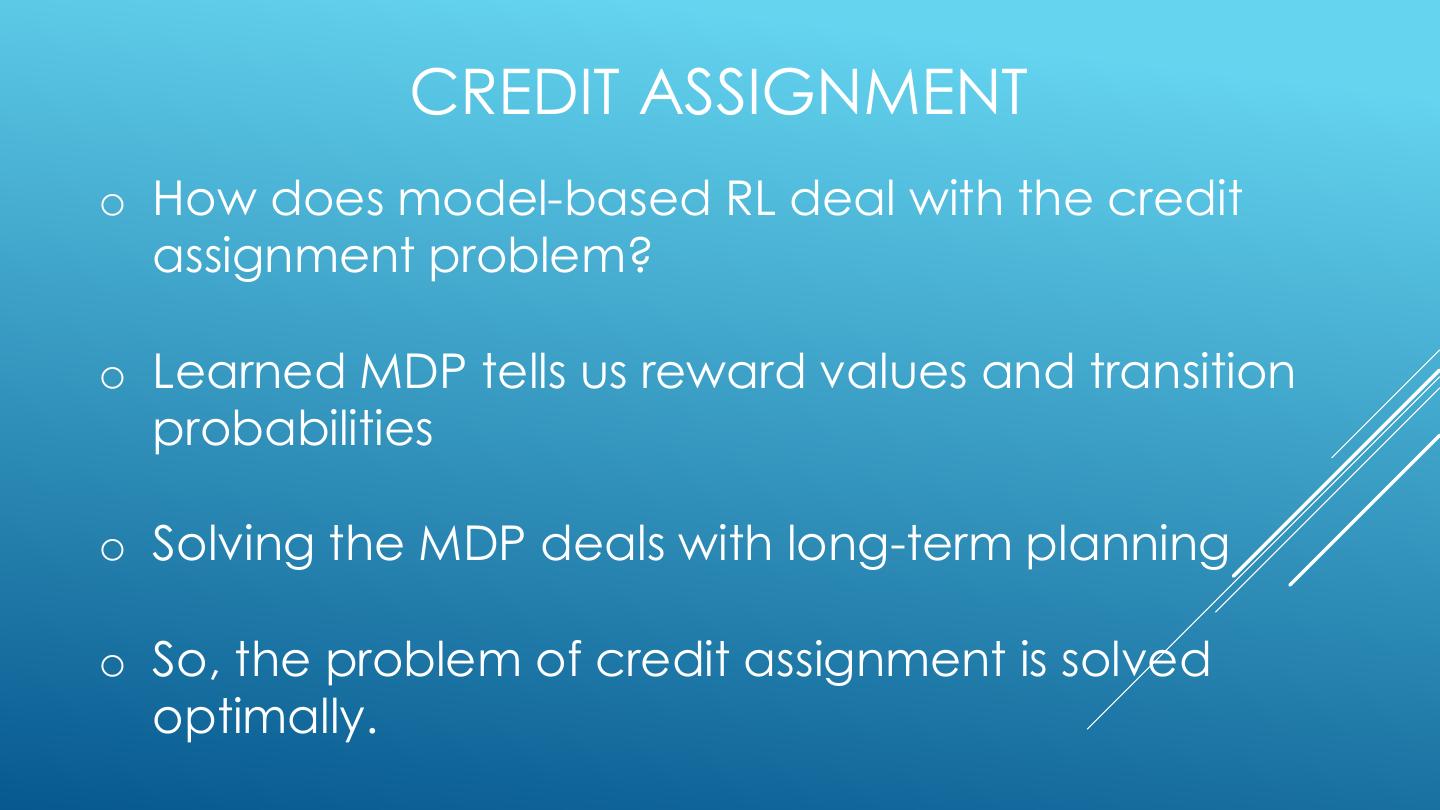
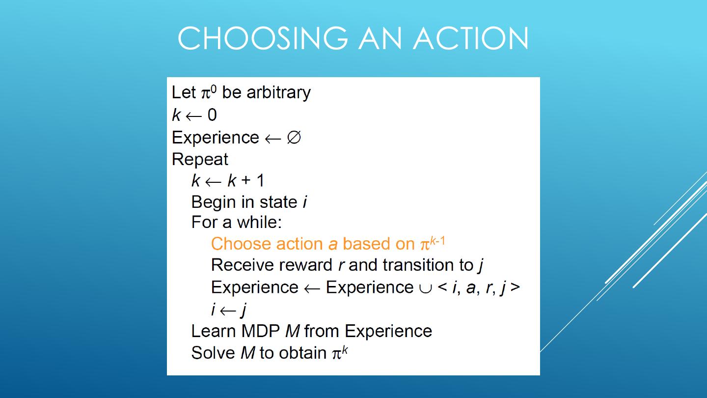
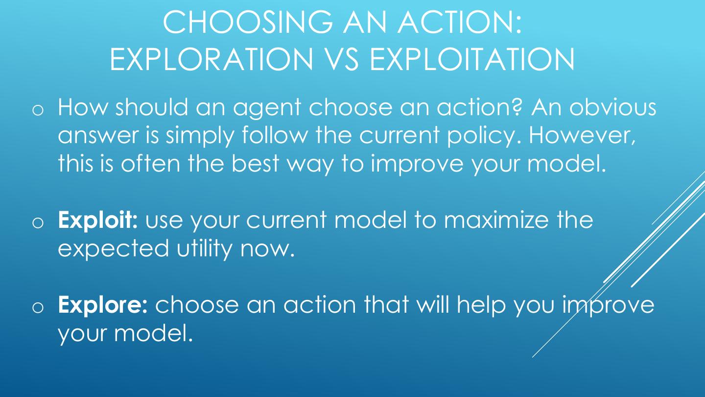
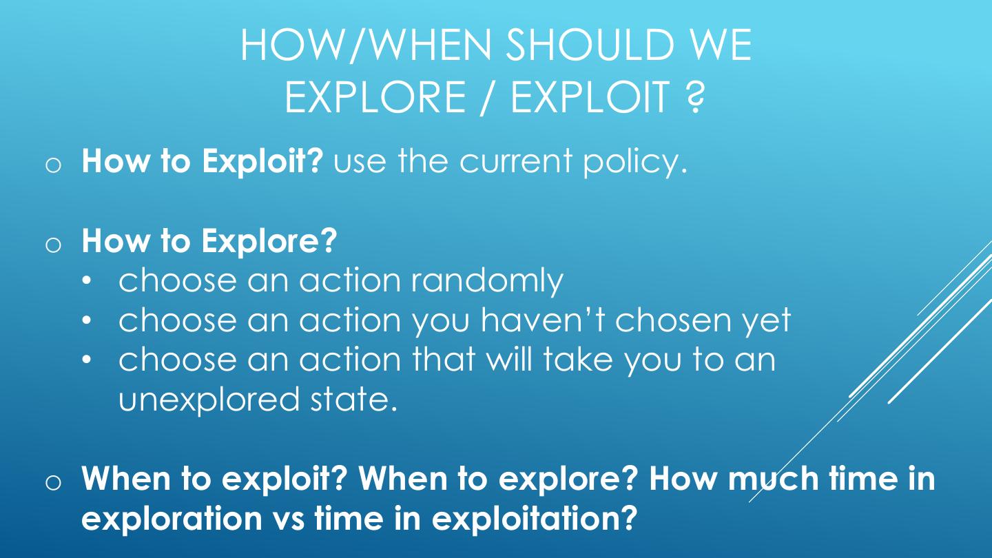
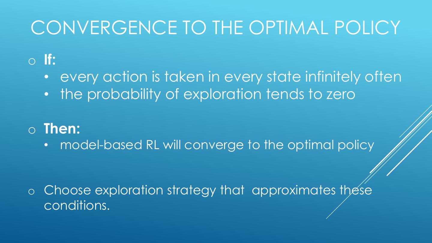
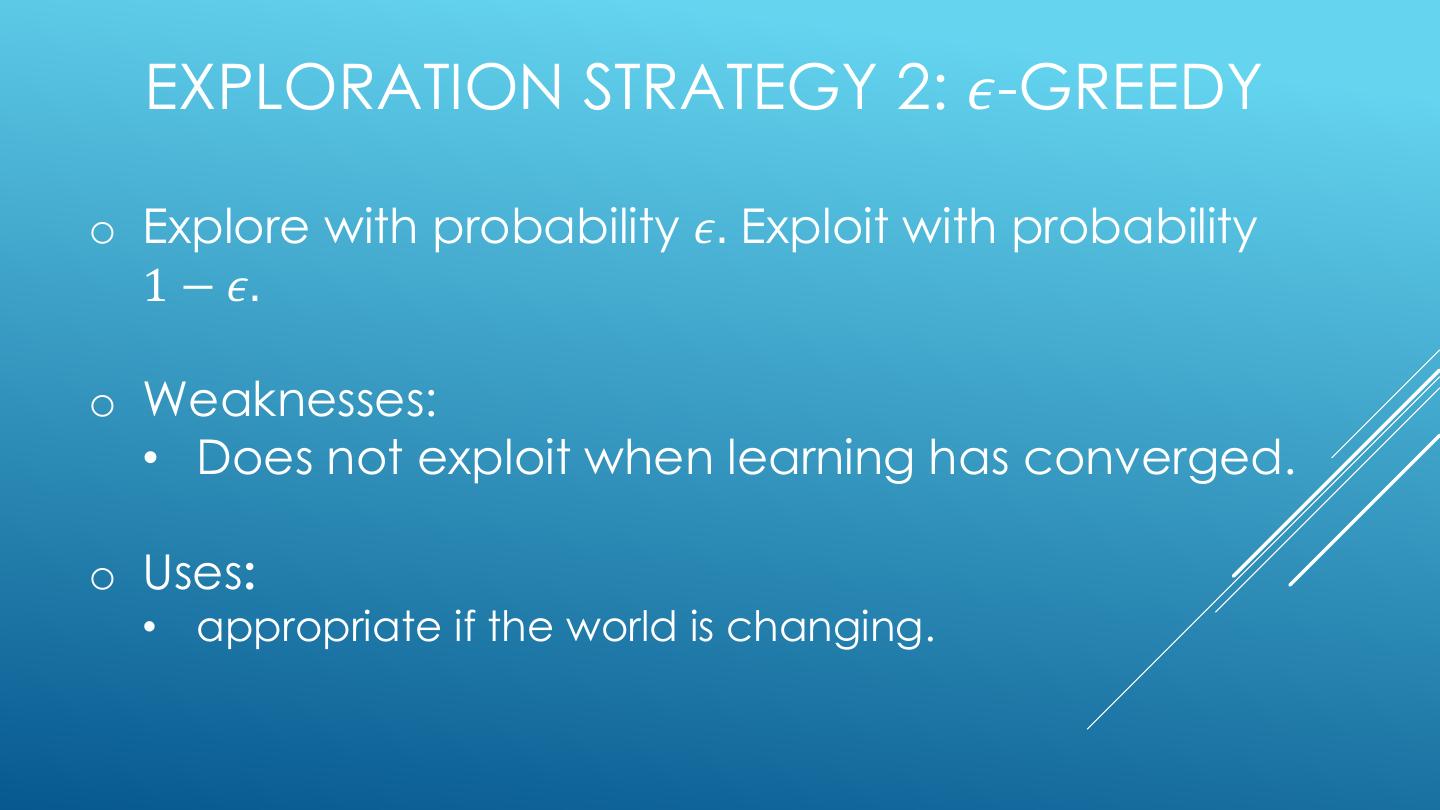
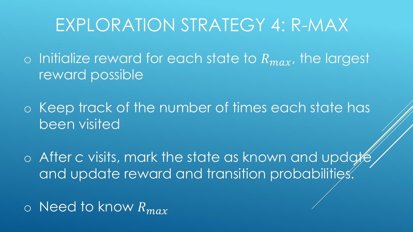
24 . CHALLENGES • credit assignment problem: how do you know which actions were responsible for success or failure? • exploration vs exploitation: should you use your current model to collect rewards or should risk lower rewards now for a better model and higher rewards later? 

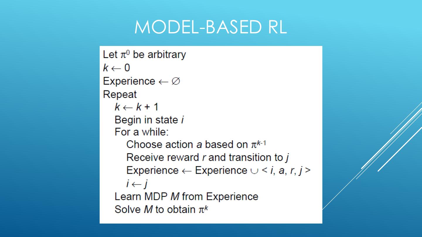
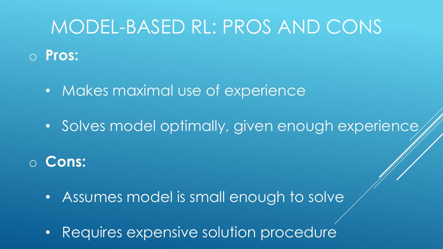
25 .MODEL-BASED REINFORCEMENT LEARNING o Mechanism is Markov Decision Process - assume states and actions are known - assume states are fully observable o Approach: - learn the MDP reward and transition parameters - solve the MDP to determine an optimal policy o Appropriate when the model is unknown, but small enough to store and solve. 

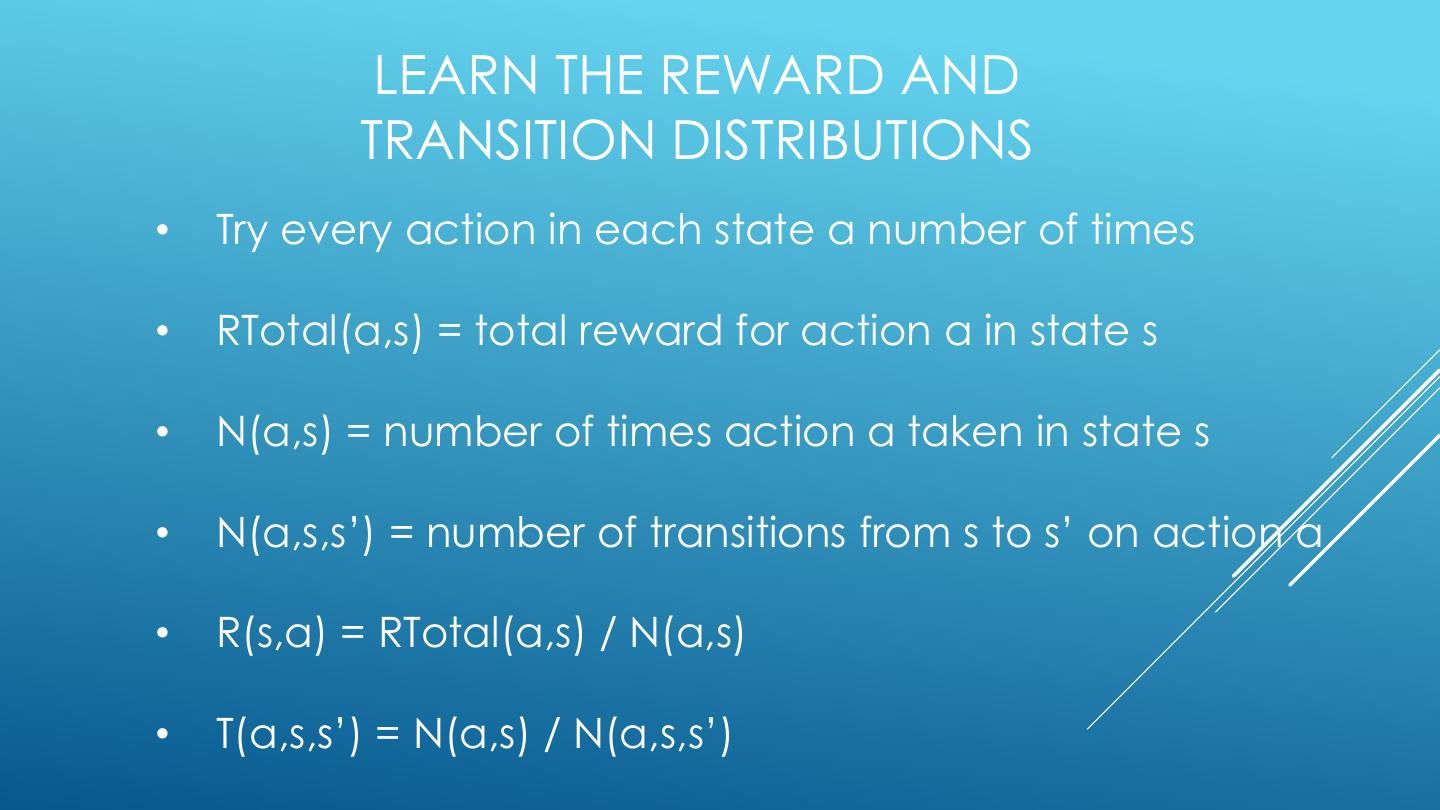
26 . LEARN THE REWARD AND TRANSITION DISTRIBUTIONS • Try every action in each state a number of times • RTotal(a,s) = total reward for action a in state s • N(a,s) = number of times action a taken in state s • N(a,s,s’) = number of transitions from s to s’ on action a • R(s,a) = RTotal(a,s) / N(a,s) • T(a,s,s’) = N(a,s) / N(a,s,s’) 

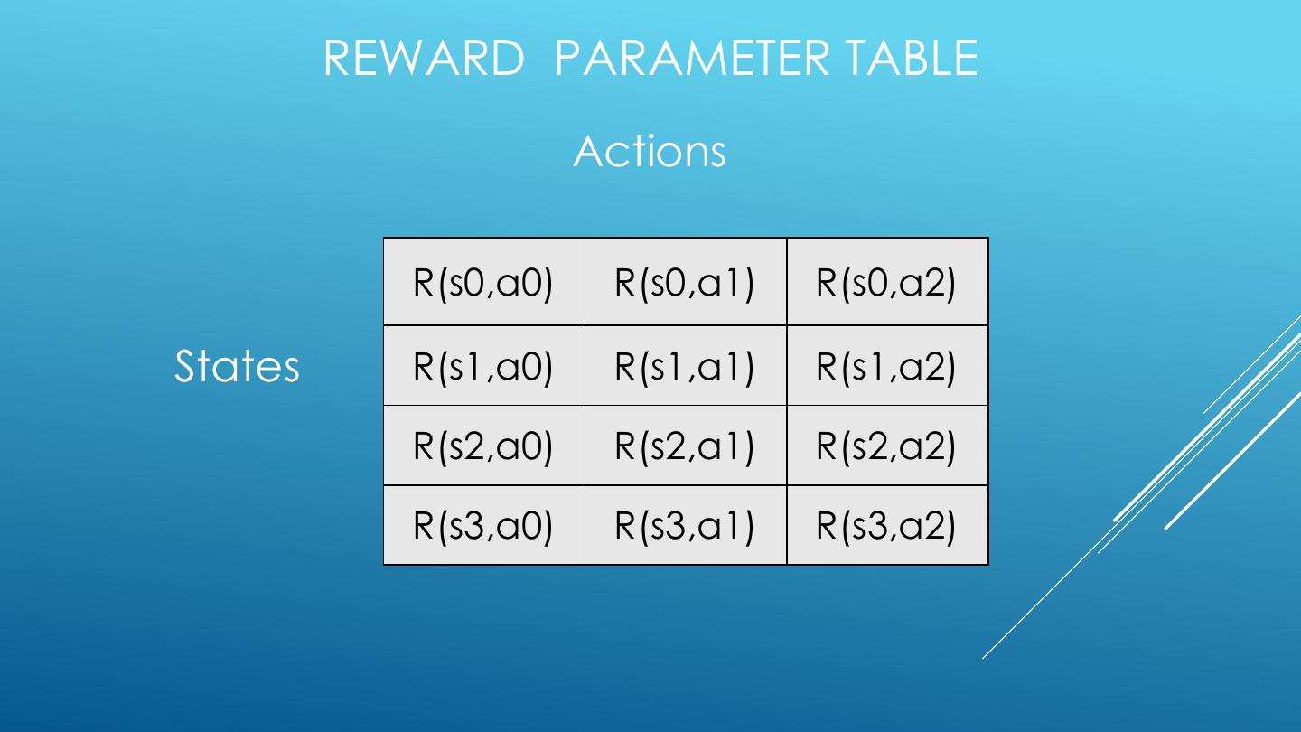
27 . REWARD PARAMETER TABLE Actions R(s0,a0) R(s0,a1) R(s0,a2) States R(s1,a0) R(s1,a1) R(s1,a2) R(s2,a0) R(s2,a1) R(s2,a2) R(s3,a0) R(s3,a1) R(s3,a2) 

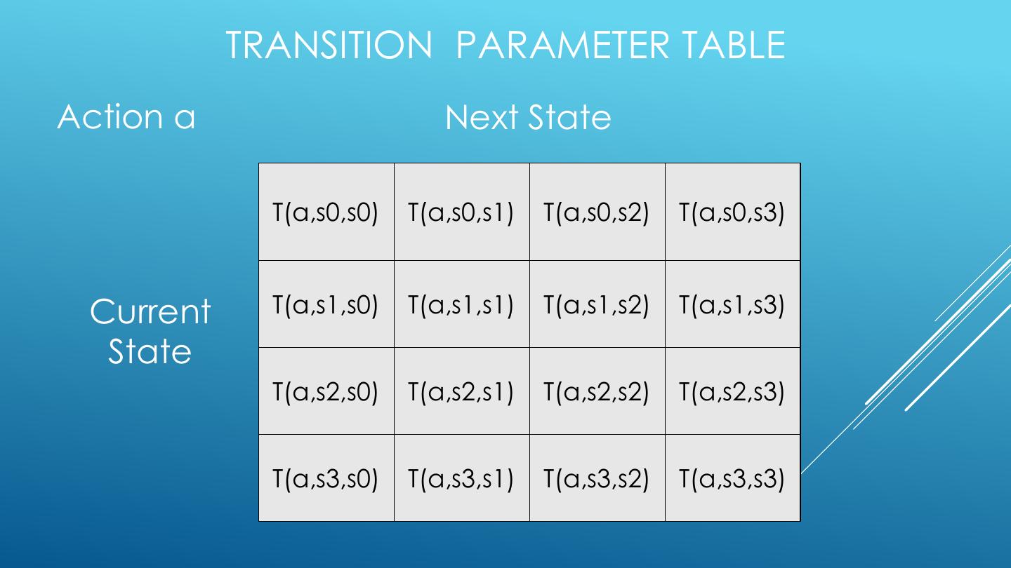
28 . TRANSITION PARAMETER TABLE Action a Next State T(a,s0,s0) T(a,s0,s1) T(a,s0,s2) T(a,s0,s3) Current T(a,s1,s0) T(a,s1,s1) T(a,s1,s2) T(a,s1,s3) State T(a,s2,s0) T(a,s2,s1) T(a,s2,s2) T(a,s2,s3) T(a,s3,s0) T(a,s3,s1) T(a,s3,s2) T(a,s3,s3) 

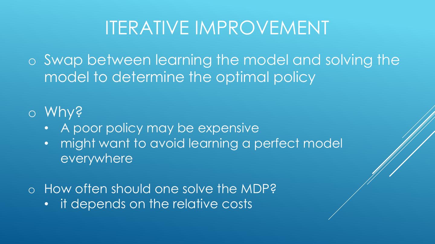
29 . ITERATIVE IMPROVEMENT o Swap between learning the model and solving the model to determine the optimal policy o Why? • A poor policy may be expensive • might want to avoid learning a perfect model everywhere o How often should one solve the MDP? • it depends on the relative costs