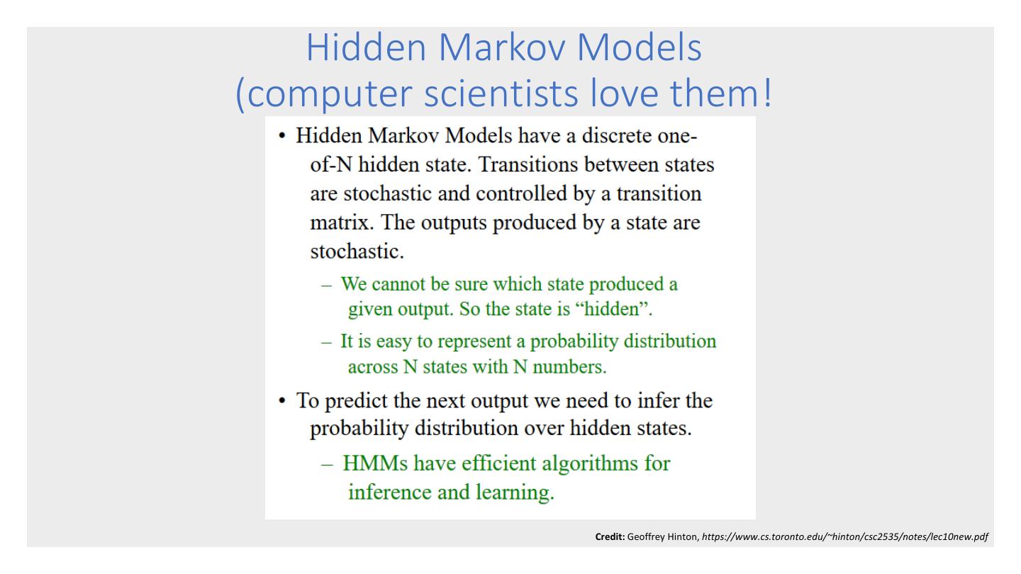
Hidden Markov Models

1 . Scott O’Hara Hidden Markov Metrowest Developers Machine Learning Group Models 05/23/2018 

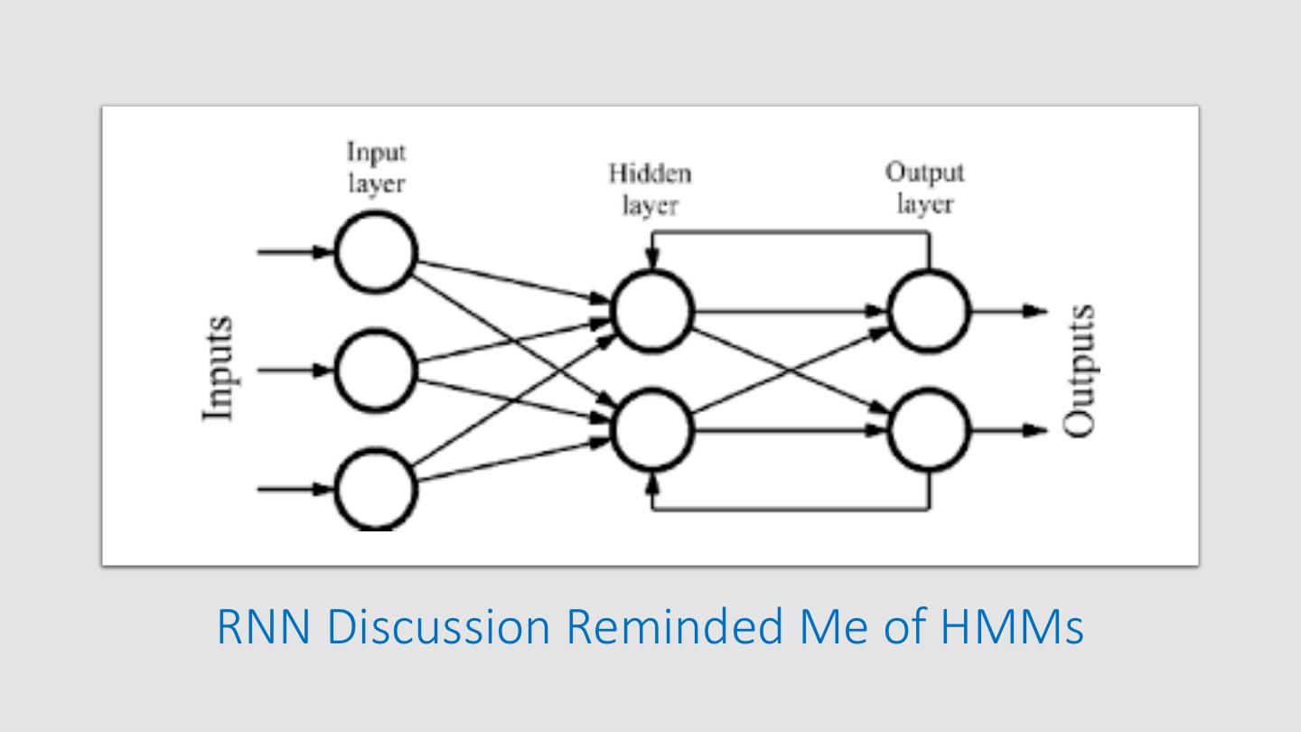
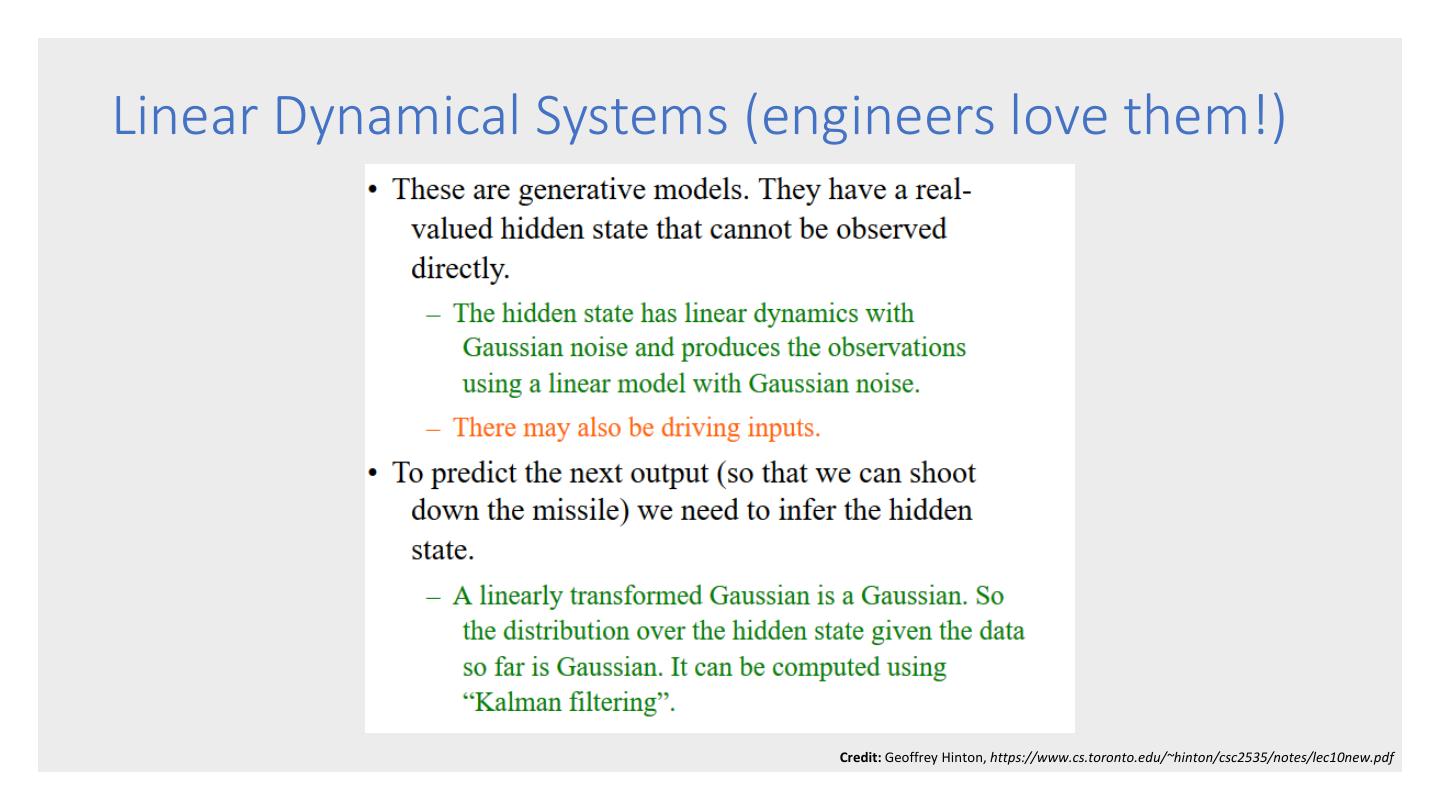
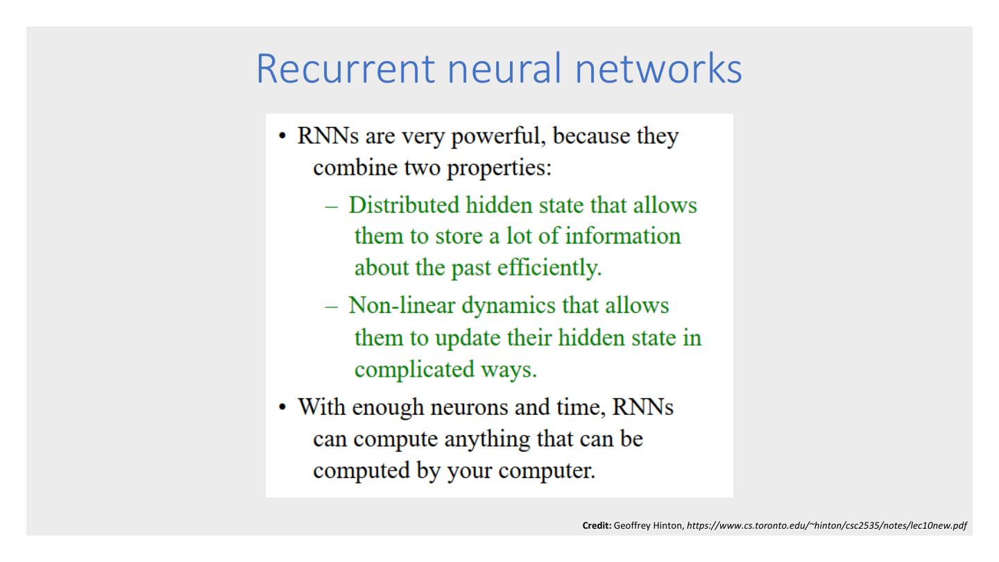
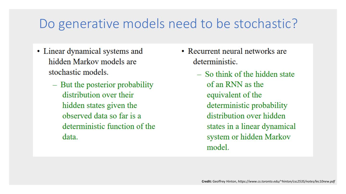
2 .RNN Discussion Reminded Me of HMMs 

3 .HMM Data Flow Choose Choose Choose Initial Next Final State State State Choose Observation State 

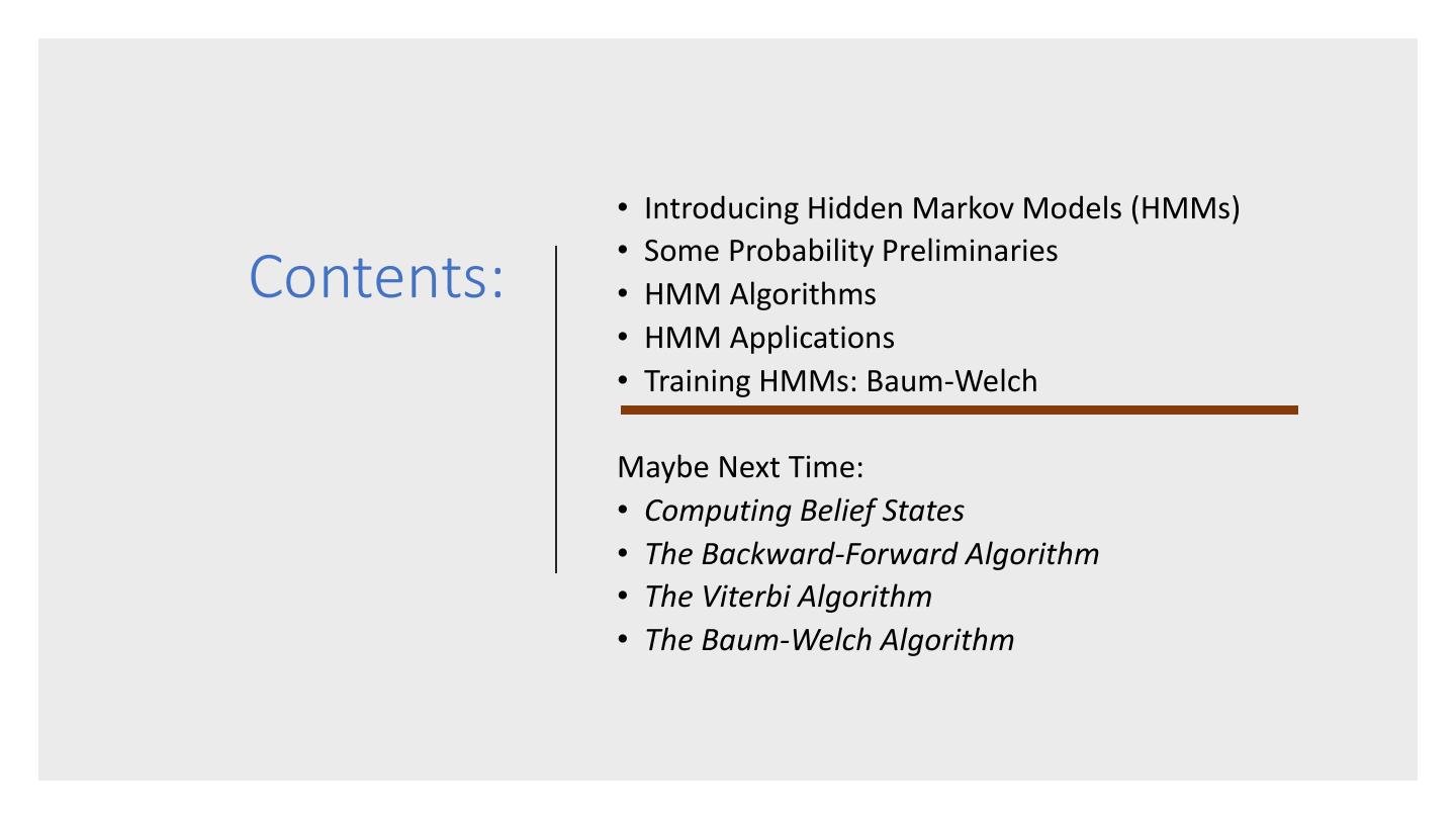
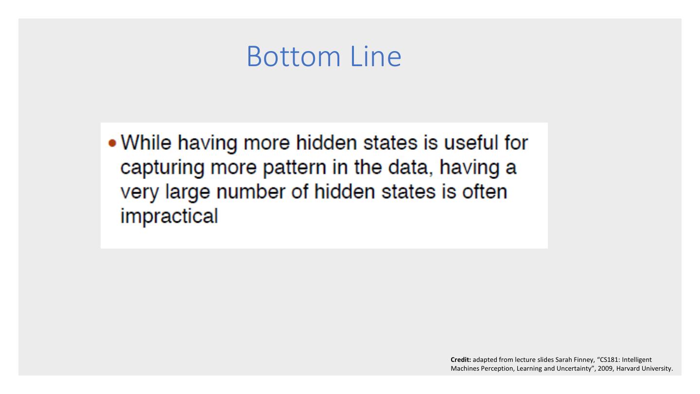
4 . • Introducing Hidden Markov Models (HMMs) • Some Probability Preliminaries Contents: • HMM Algorithms • HMM Applications • Training HMMs: Baum-Welch Maybe Next Time: • Computing Belief States • The Backward-Forward Algorithm • The Viterbi Algorithm • The Baum-Welch Algorithm 

5 .Introducing Hidden Markov Models • Markov Processes • Hidden Markov Models (HMM) • The Markov Assumptions 

6 . • A Markov process (or chain) is a stochastic model describing a sequence of possible events in which the probability of each event depends only on the state attained in the previous event. Source: https://en.oxforddictionaries.com/definition/us/markov_chain Markov Process • A Markov process has the following components: • A set of N states • A transition probability matrix representing the probability of moving from state i to state j. . For any state i, all probabilities must sum to 1. • A special start state and end state. Source: adapted from https://web.stanford.edu/~jurafsky/slp3/9.pdf 

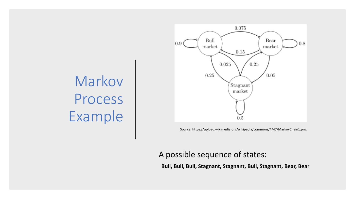
7 . Markov Process Example Source: https://upload.wikimedia.org/wikipedia/commons/4/47/MarkovChain1.png A possible sequence of states: Bull, Bull, Bull, Stagnant, Stagnant, Bull, Stagnant, Bear, Bear 

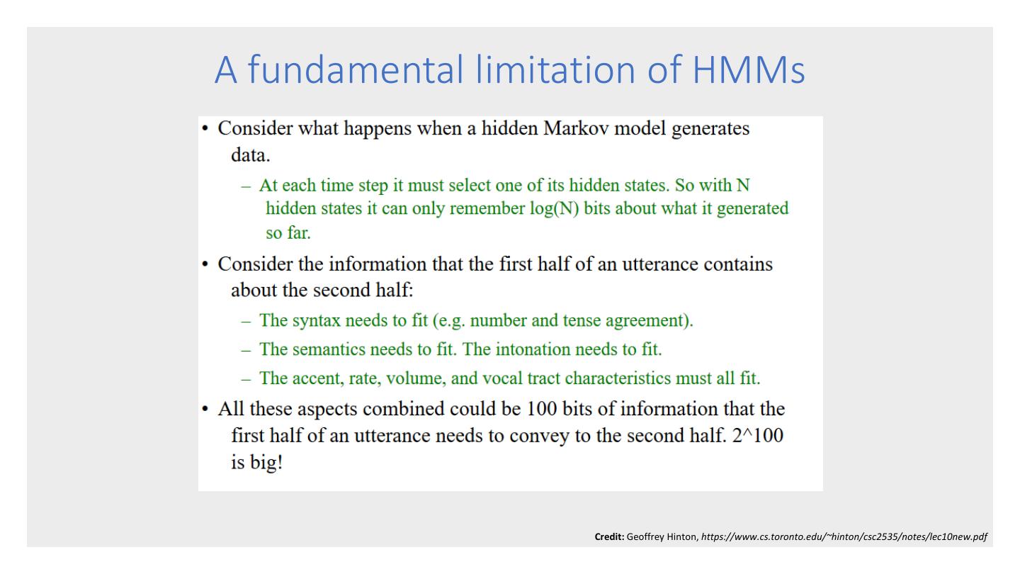
8 . • A Hidden Markov Model (HMM) is a statistical model in which the system being modeled is assumed to be a Markov process with unobserved (i.e. hidden) states. Source: https://en.wikipedia.org/wiki/Hidden_Markov_model • A Hidden Markov model has the following components: • A set of N states Hidden • An initial probability distribution over the states specifying the probability that state i is the first Markov state in a sequence. • A transition probability matrix representing the Models probability of moving from state i to state j. . For any state i, all probabilities must sum to 1. • A sequence of observation states. • a sequence of observation likelihoods each expressing the probability of an observation i being generated from state i. Source: adapted from https://web.stanford.edu/~jurafsky/slp3/9.pdf 

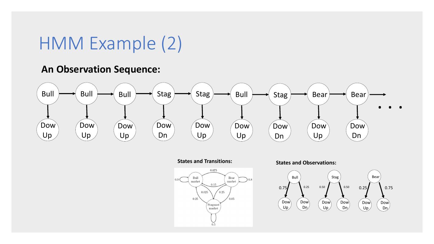
9 .HMM Example (1) States and Transitions: States and Observations: Bull Stag Bear 0.75 0.25 0.50 0.50 0.25 0.75 Dow Dow Dow Dow Dow Dow Up Dn Up Dn Up Dn 

10 .HMM Example (2) An Observation Sequence: Bull Bull Bull Stag Stag Bull Stag Bear Bear ... Dow Dow Dow Dow Dow Dow Dow Dow Dow Up Up Up Dn Up Up Dn Up Dn States and Transitions: States and Observations: Bull Stag Bear 0.75 0.25 0.50 0.50 0.25 0.75 Dow Dow Dow Dow Dow Dow Up Dn Up Dn Up Dn 

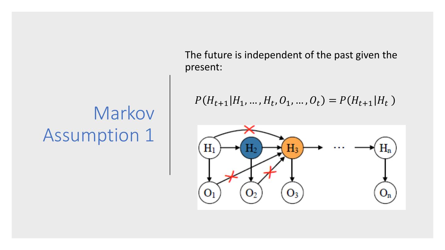
11 . The future is independent of the past given the present: 𝑃 𝐻𝑡+1 𝐻1 , … , 𝐻𝑡 , 𝑂1 , … , 𝑂𝑡 = 𝑃 𝐻𝑡+1 𝐻𝑡 Markov Assumption 1 

12 . Observations depend only on the current hidden state: 𝑃 𝑂𝑡 𝐻1 , … , 𝐻𝑡 , 𝑂1 , … , 𝑂𝑡 = 𝑃 𝑂𝑡 𝐻𝑡 Markov Assumption 2 

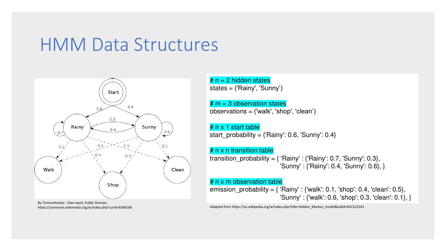
13 . HMM Data Structures # n = 2 hidden states states = ('Rainy', 'Sunny’) # m = 3 observation states observations = ('walk', 'shop', 'clean’) # n x 1 start table start_probability = {'Rainy': 0.6, 'Sunny': 0.4} # n x n transition table transition_probability = { 'Rainy' : {'Rainy': 0.7, 'Sunny': 0.3}, 'Sunny' : {'Rainy': 0.4, 'Sunny': 0.6}, } # n x m observation table emission_probability = { 'Rainy' : {'walk': 0.1, 'shop': 0.4, 'clean': 0.5}, 'Sunny' : {'walk': 0.6, 'shop': 0.3, 'clean': 0.1}, } By Terencehonles - Own work, Public Domain, https://commons.wikimedia.org/w/index.php?curid=8384168 Adapted from https://en.wikipedia.org/w/index.php?title=Hidden_Markov_model&oldid=841523243 

14 .Some Probability Preliminaries 

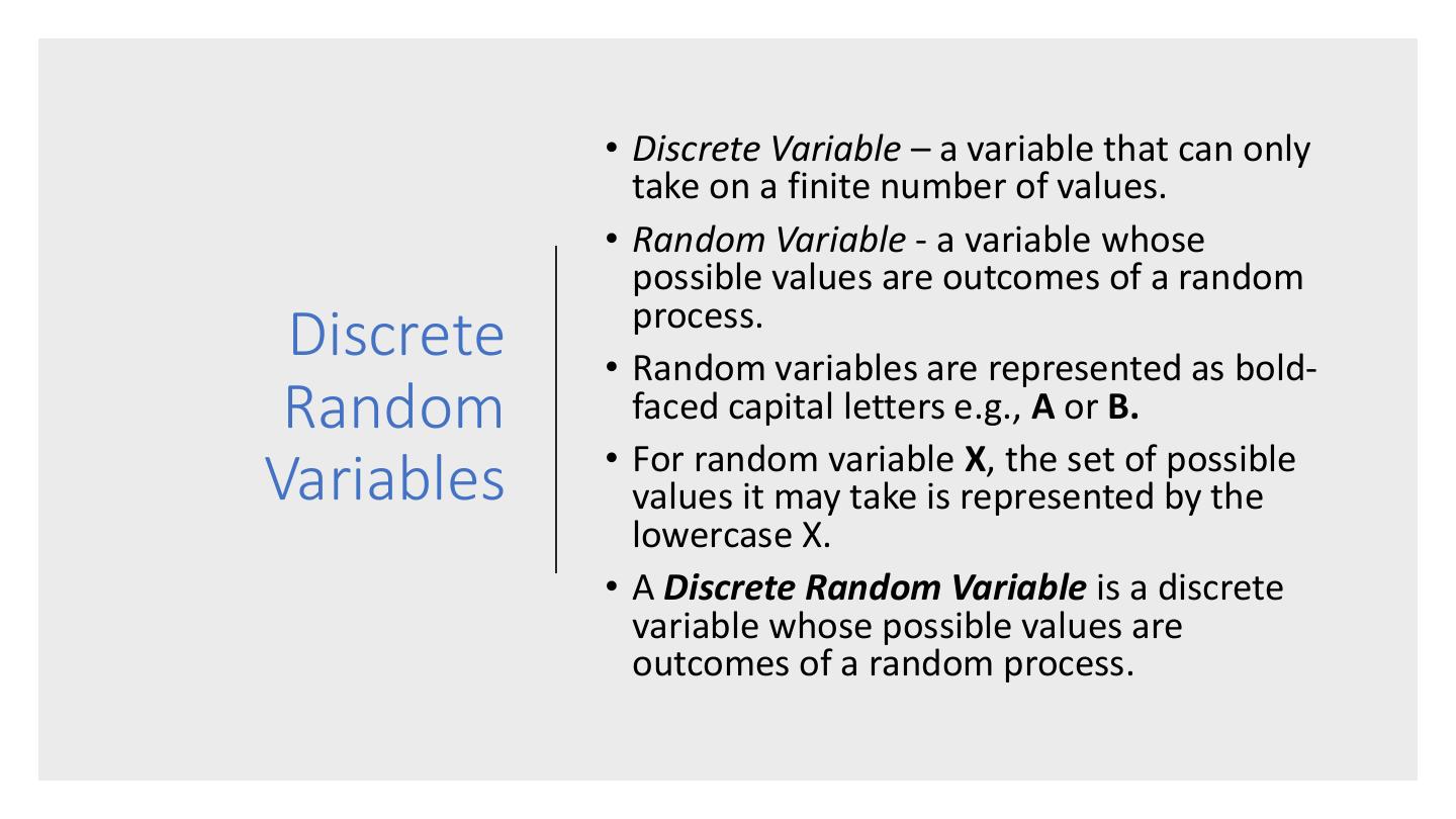
15 . • Discrete Random Variables • Probabilities and the Sum Rule • Joint Probability Some • Conditional Probability Probability • The Product Rule Preliminaries • The Chain Rule • Bayes’ Rule • Marginalization 

16 . • Discrete Variable – a variable that can only take on a finite number of values. • Random Variable - a variable whose possible values are outcomes of a random process. Discrete • Random variables are represented as bold- Random faced capital letters e.g., A or B. • For random variable X, the set of possible Variables values it may take is represented by the lowercase X. • A Discrete Random Variable is a discrete variable whose possible values are outcomes of a random process. 

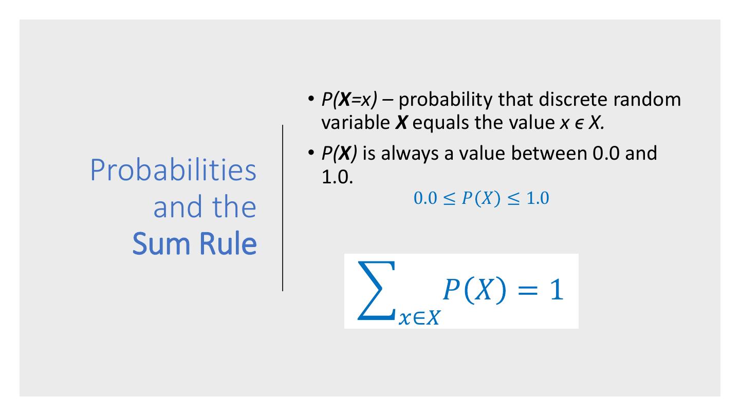
17 . • P(X=x) – probability that discrete random variable X equals the value x ϵ X. • P(X) is always a value between 0.0 and Probabilities 1.0. 0.0 ≤ 𝑃 𝑋 ≤ 1.0 and the Sum Rule ෍ 𝑃 𝑋 =1 𝑥∈𝑋 

18 . World Joint Probability P(a) P(b) Identities: P(A,B) = P(B,A) P(a,b) 

19 . World Conditional Probability P(a) P(b) P(A|B) – What is the probability that A is P(a|b) true given that B is true? Identities: 𝑃 𝑨,𝑩 P 𝑨𝑩 = 𝑃 𝑩 

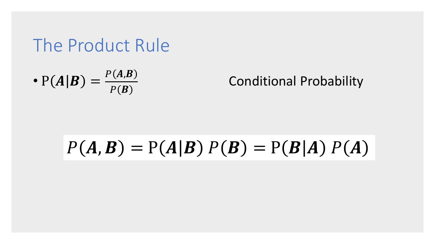
20 .The Product Rule 𝑃 𝑨,𝑩 •P 𝑨 𝑩 = Conditional Probability 𝑃 𝑩 𝑃 𝑨, 𝑩 = P 𝑨 𝑩 𝑃 𝑩 = P 𝑩 𝑨 𝑃 𝑨 

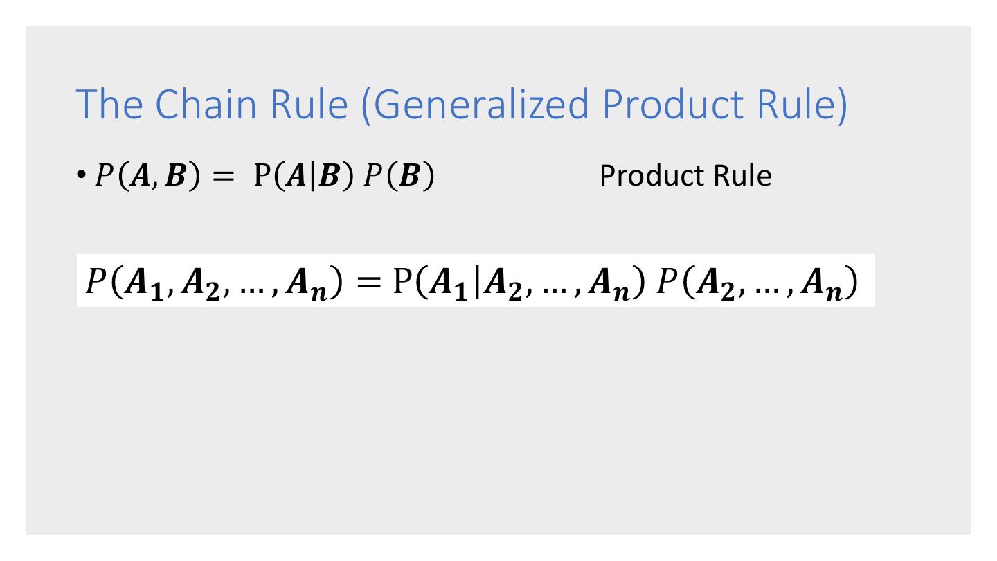
21 .The Chain Rule (Generalized Product Rule) • 𝑃 𝑨, 𝑩 = P 𝑨 𝑩 𝑃 𝑩 Product Rule 𝑃 𝑨𝟏 , 𝑨𝟐 , … , 𝑨𝒏 = P 𝑨𝟏 𝑨𝟐 , … , 𝑨𝒏 𝑃 𝑨𝟐 , … , 𝑨𝒏 

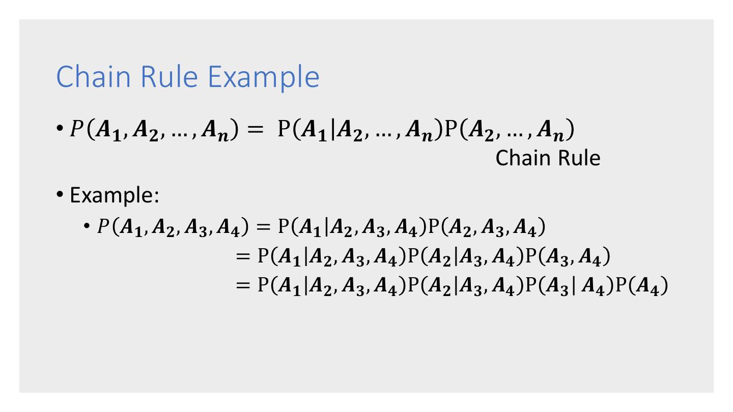
22 .Chain Rule Example • 𝑃 𝑨𝟏 , 𝑨𝟐 , … , 𝑨𝒏 = P 𝑨𝟏 𝑨𝟐 , … , 𝑨𝒏 P 𝑨𝟐 , … , 𝑨𝒏 Chain Rule • Example: • 𝑃 𝑨𝟏 , 𝑨𝟐 , 𝑨𝟑 , 𝑨𝟒 = P 𝑨𝟏 𝑨𝟐 , 𝑨𝟑 , 𝑨𝟒 P 𝑨𝟐 , 𝑨𝟑 , 𝑨𝟒 = P 𝑨𝟏 𝑨𝟐 , 𝑨𝟑 , 𝑨𝟒 P 𝑨𝟐 𝑨𝟑 , 𝑨𝟒 P 𝑨𝟑 , 𝑨𝟒 = P 𝑨𝟏 𝑨𝟐 , 𝑨𝟑 , 𝑨𝟒 P 𝑨𝟐 𝑨𝟑 , 𝑨𝟒 P 𝑨𝟑 𝑨𝟒 P 𝑨𝟒 

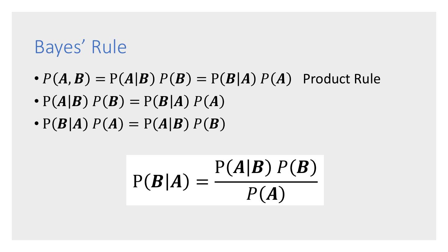
23 .Bayes’ Rule • 𝑃 𝑨, 𝑩 = P 𝑨 𝑩 𝑃 𝑩 = P 𝑩 𝑨 𝑃 𝑨 Product Rule •P 𝑨 𝑩 𝑃 𝑩 =P 𝑩 𝑨 𝑃 𝑨 •P 𝑩 𝑨 𝑃 𝑨 = P 𝑨 𝑩 𝑃 𝑩 P 𝑨𝑩 𝑃 𝑩 P 𝑩𝑨 = 𝑃 𝑨 

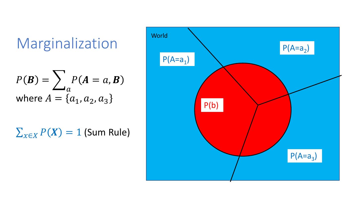
24 . World Marginalization P(A=a2) P(A=a1) 𝑃 𝑩 = ෍ 𝑃 𝑨 = 𝑎, 𝑩 𝑎 where 𝐴 = 𝑎1 , 𝑎2 , 𝑎3 P(b) σ𝑥∈𝑋 𝑃 𝑿 = 1 (Sum Rule) P(b) P(A=a3) 

25 .HMM Algorithms 

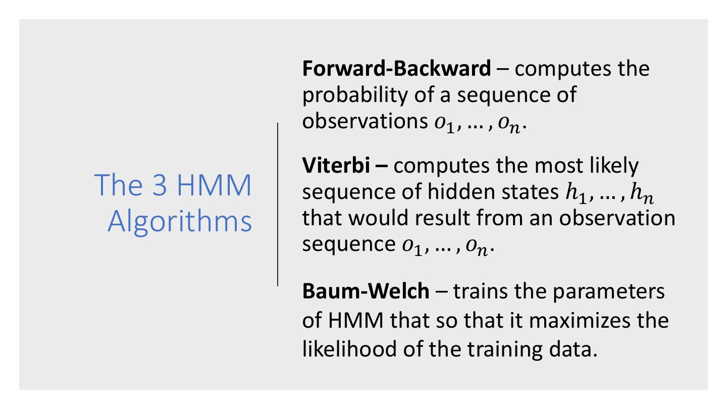
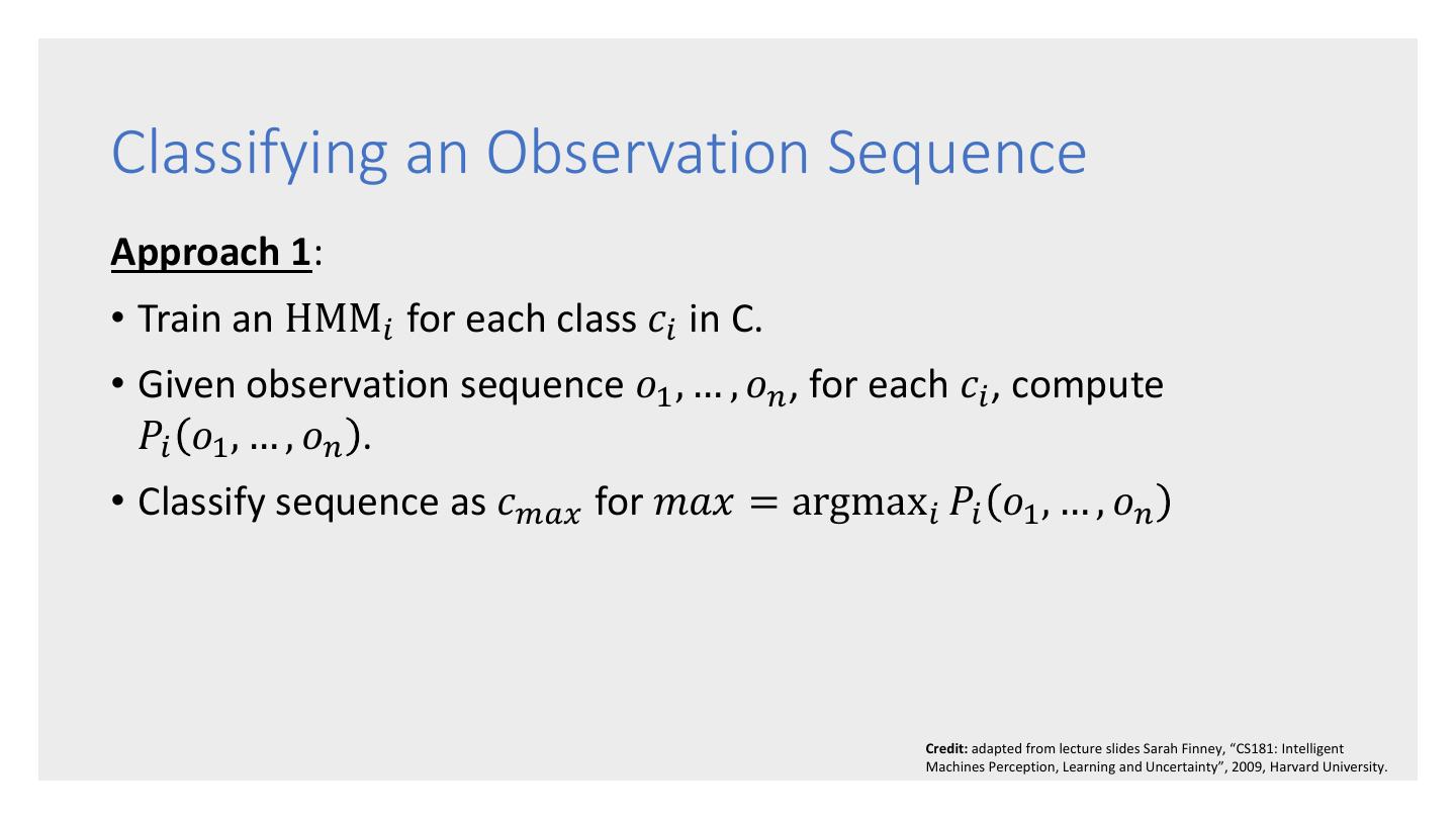
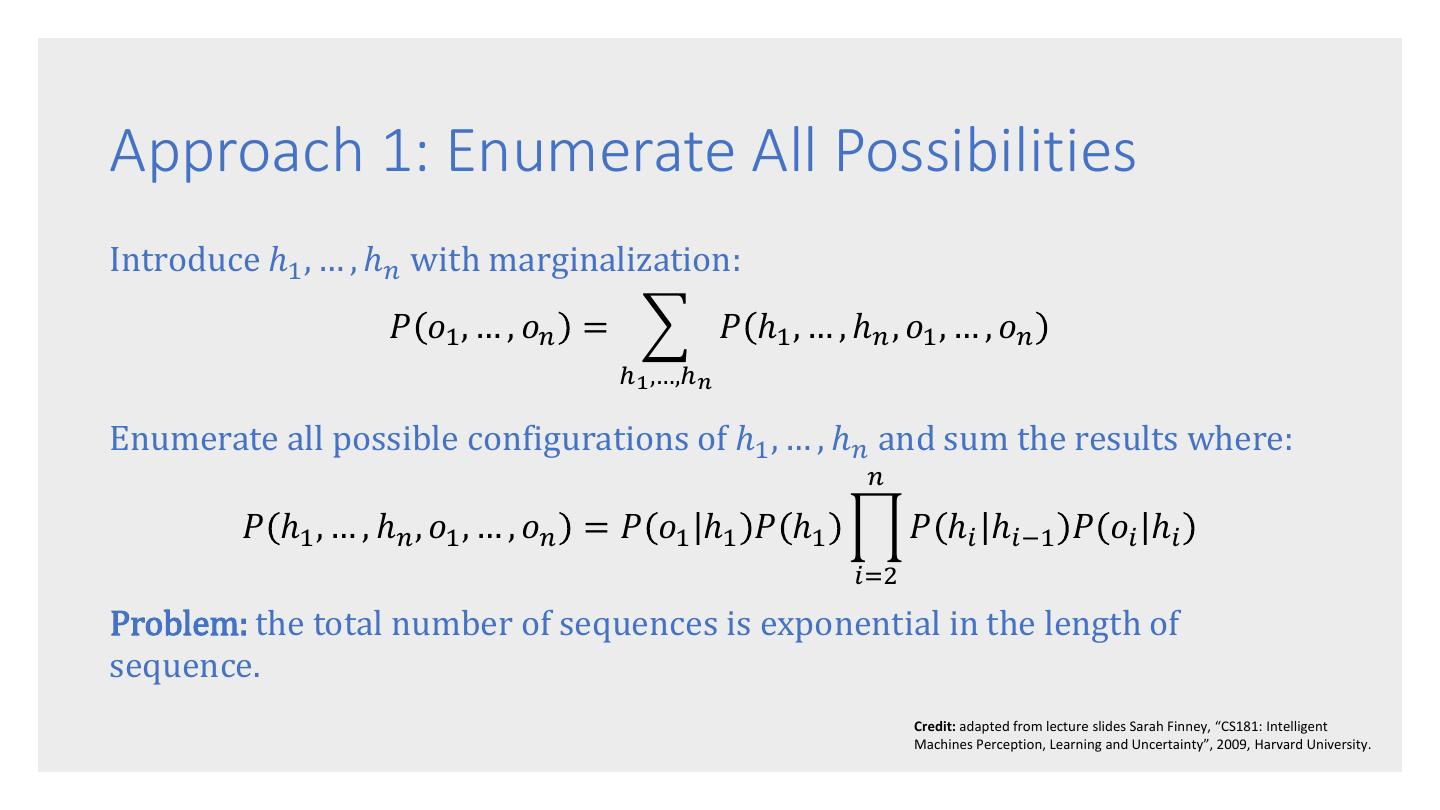
26 . Forward-Backward – computes the probability of a sequence of observations 𝑜1 , … , 𝑜𝑛 . Viterbi – computes the most likely The 3 HMM sequence of hidden states ℎ1 , … , ℎ𝑛 Algorithms that would result from an observation sequence 𝑜1 , … , 𝑜𝑛 . Baum-Welch – trains the parameters of HMM that so that it maximizes the likelihood of the training data. 

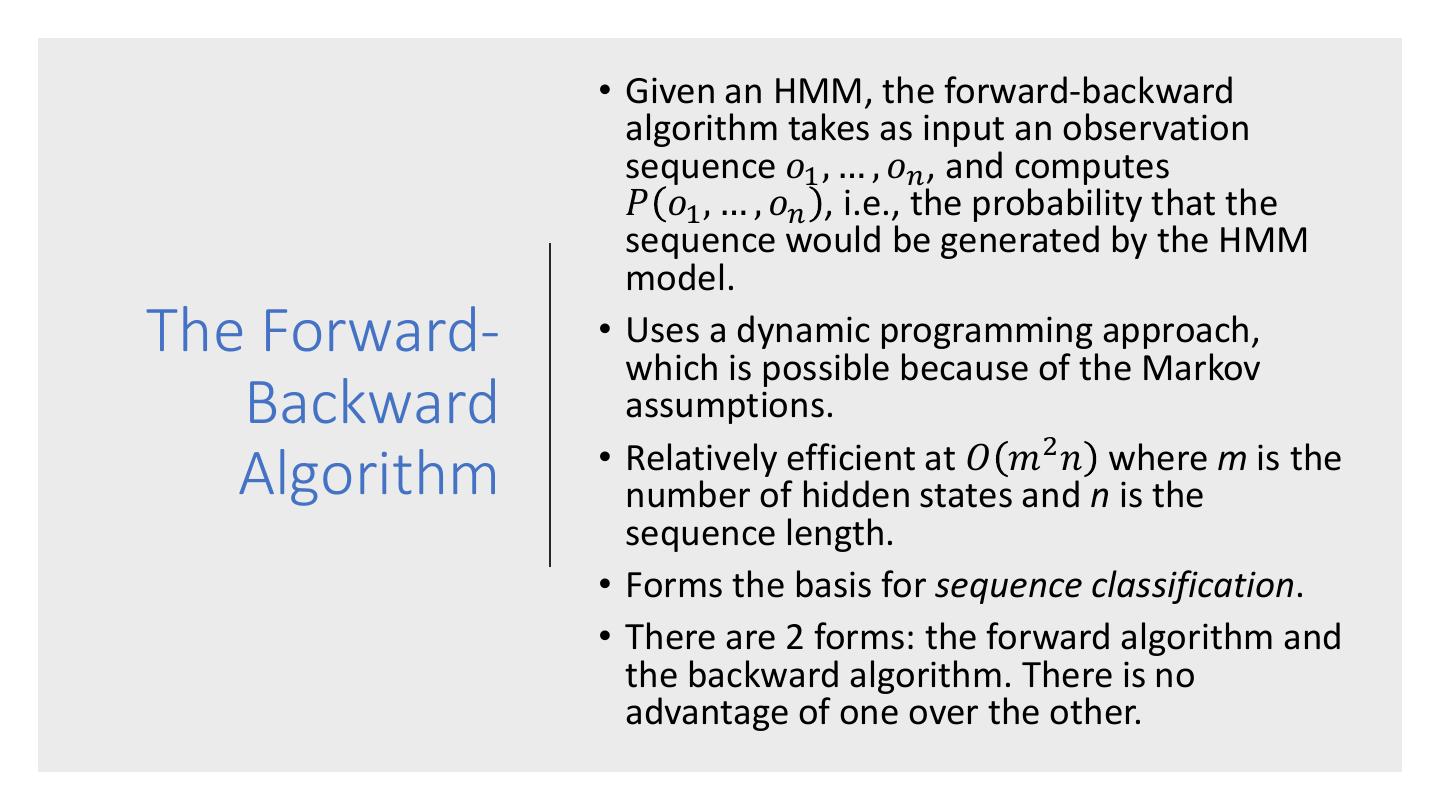
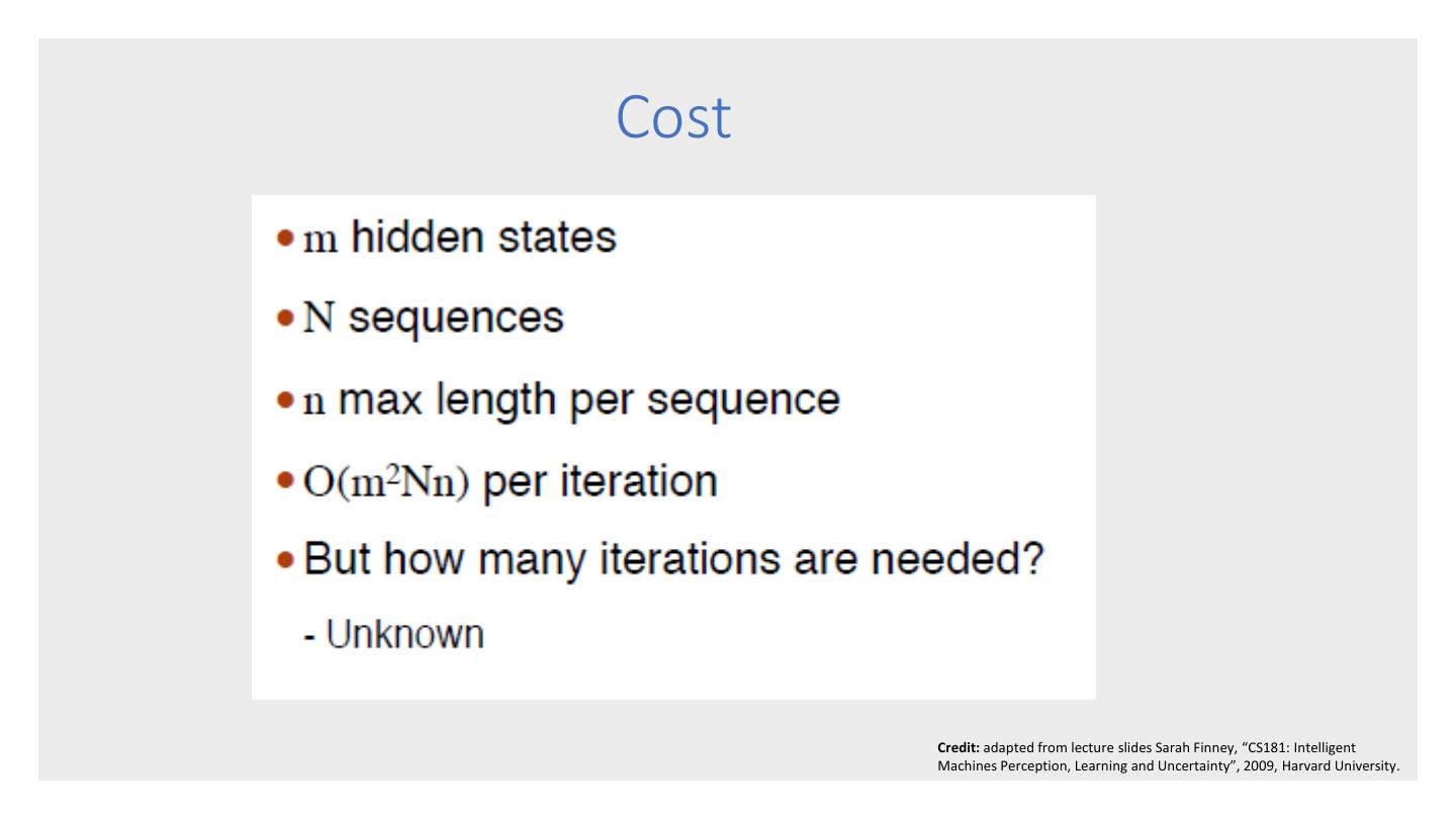
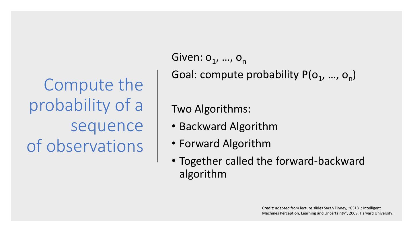
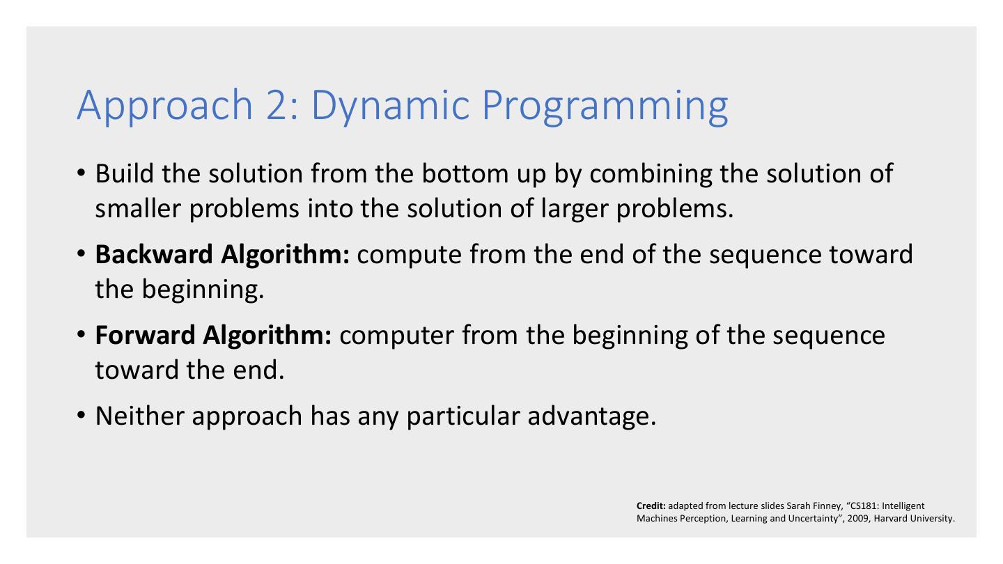
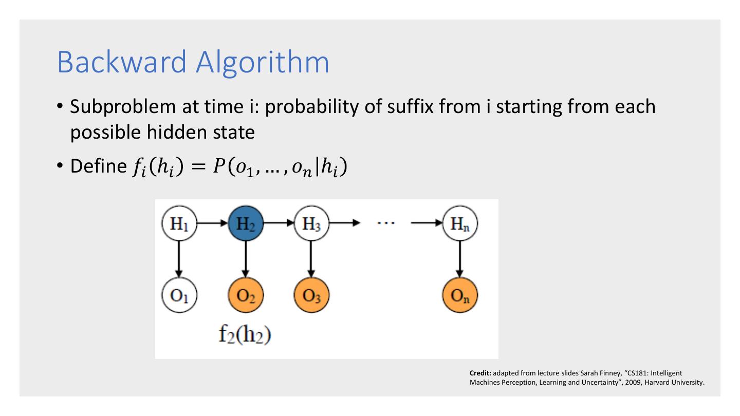
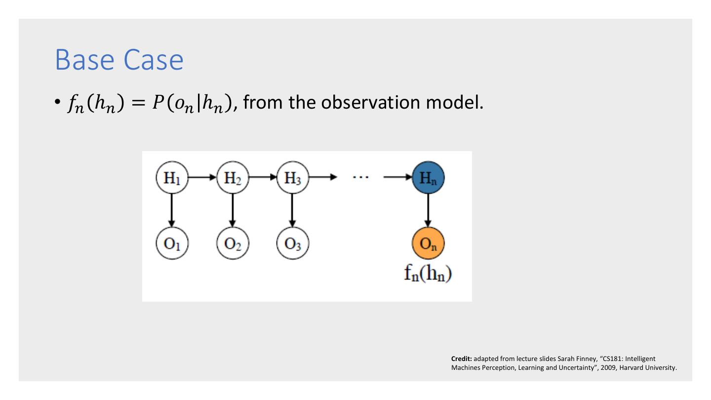
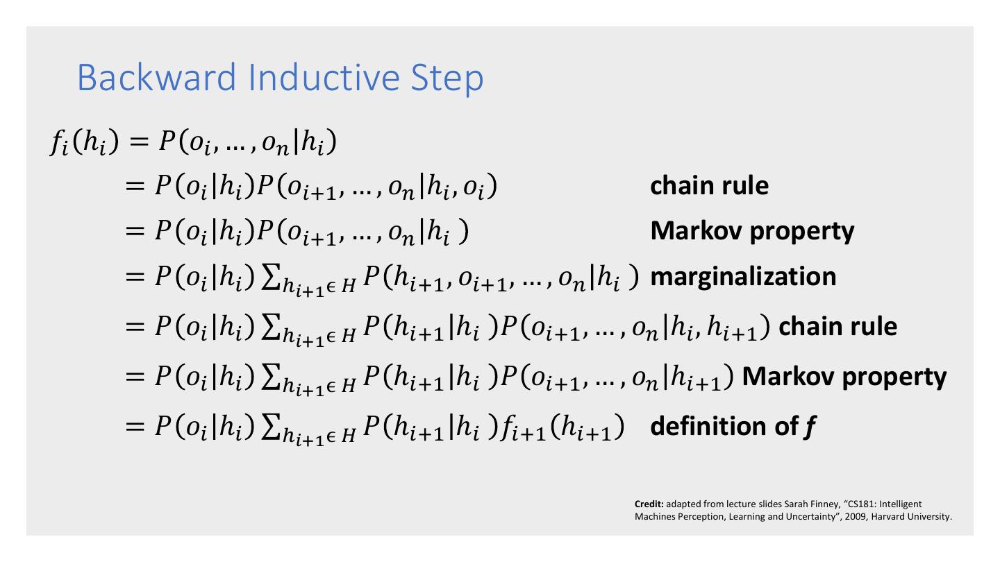
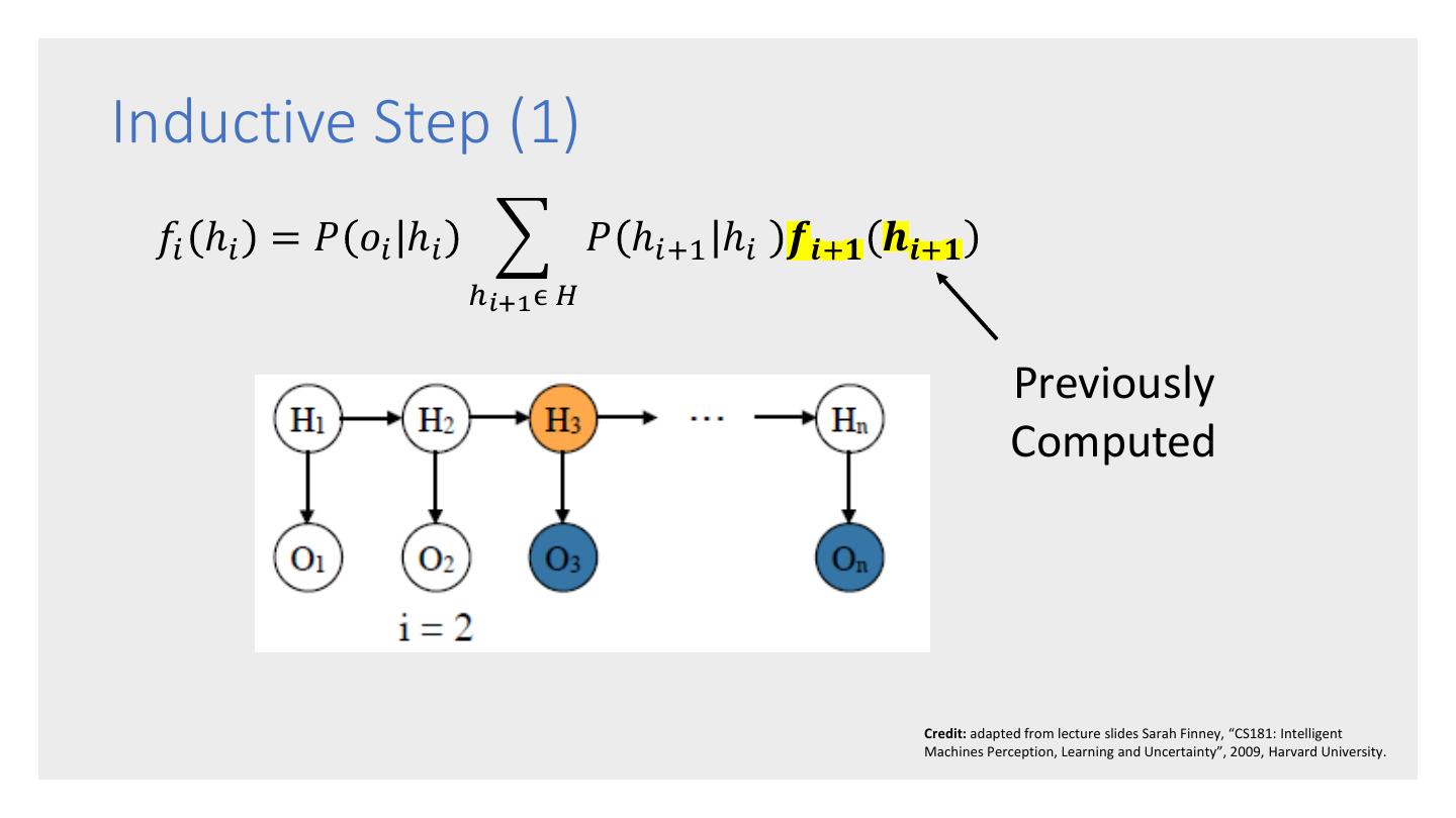
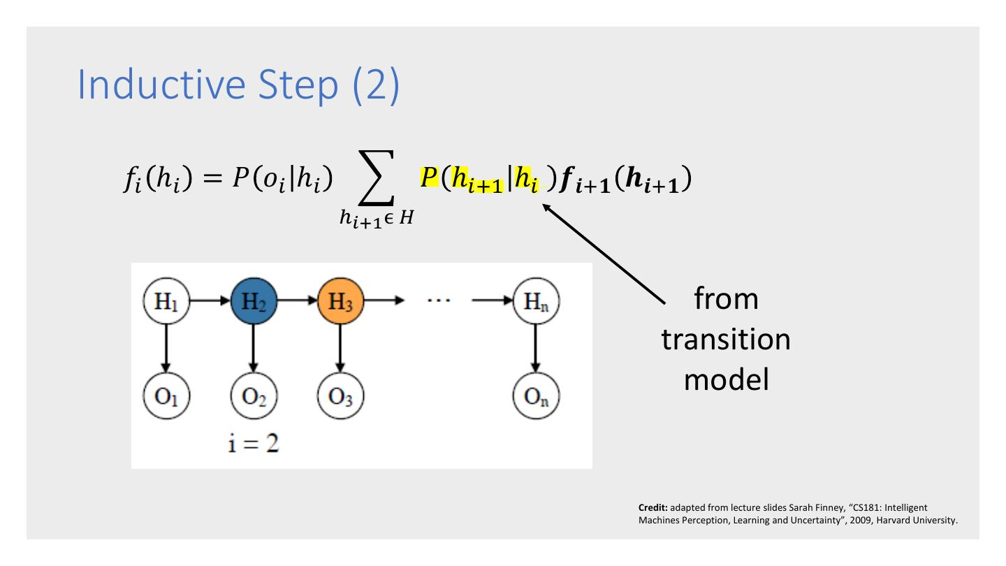
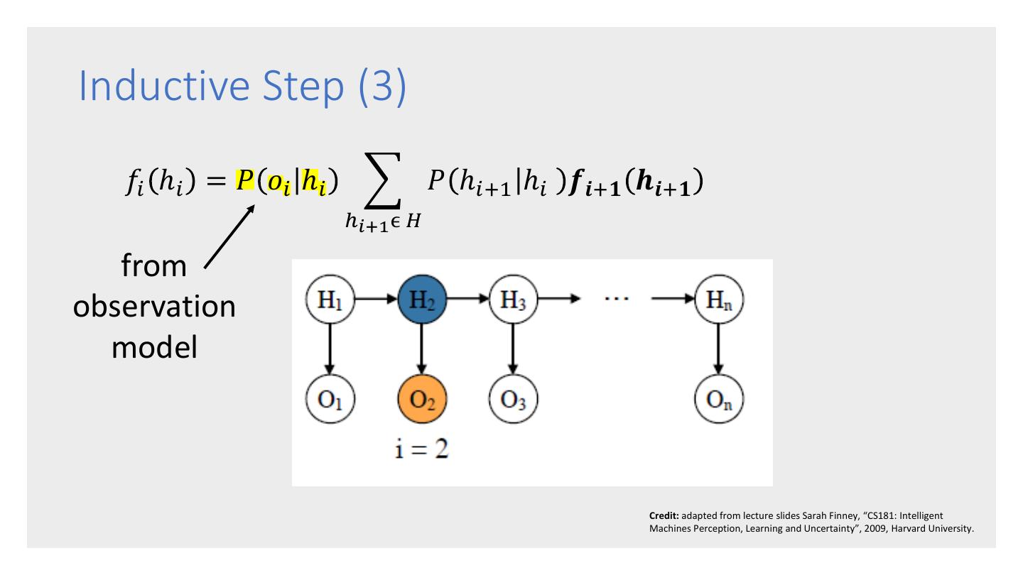
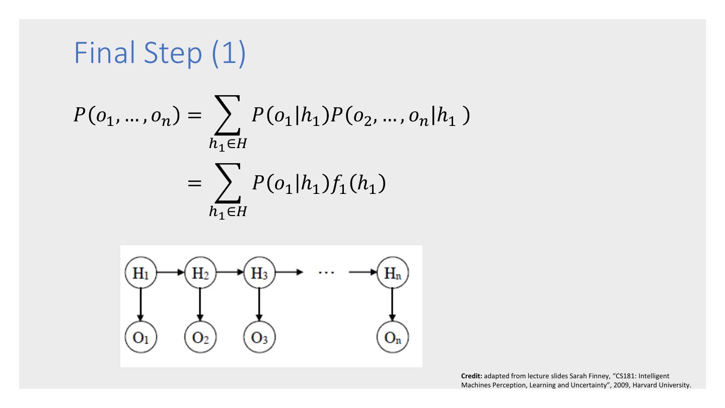
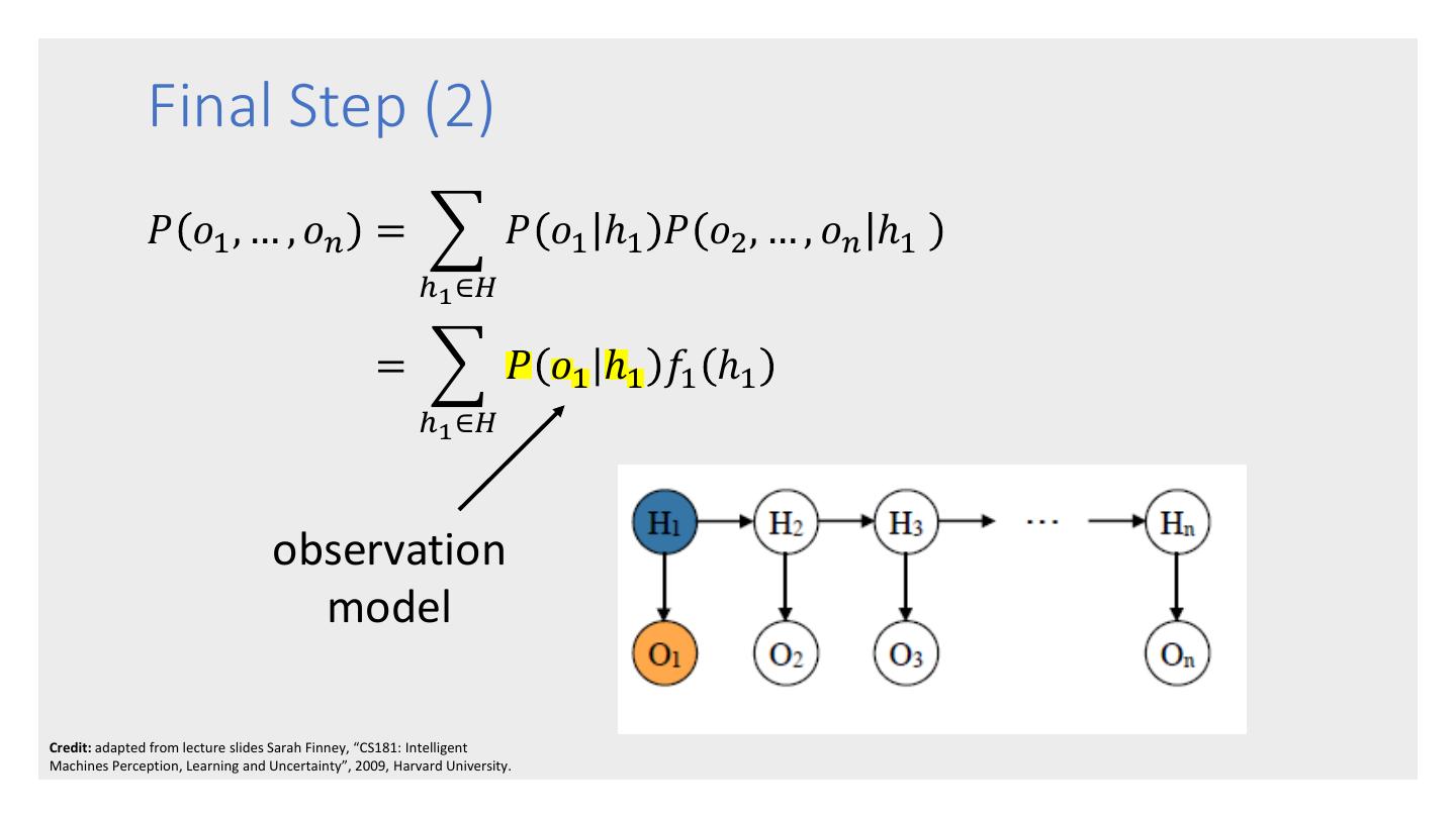
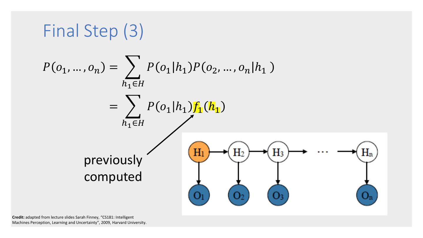
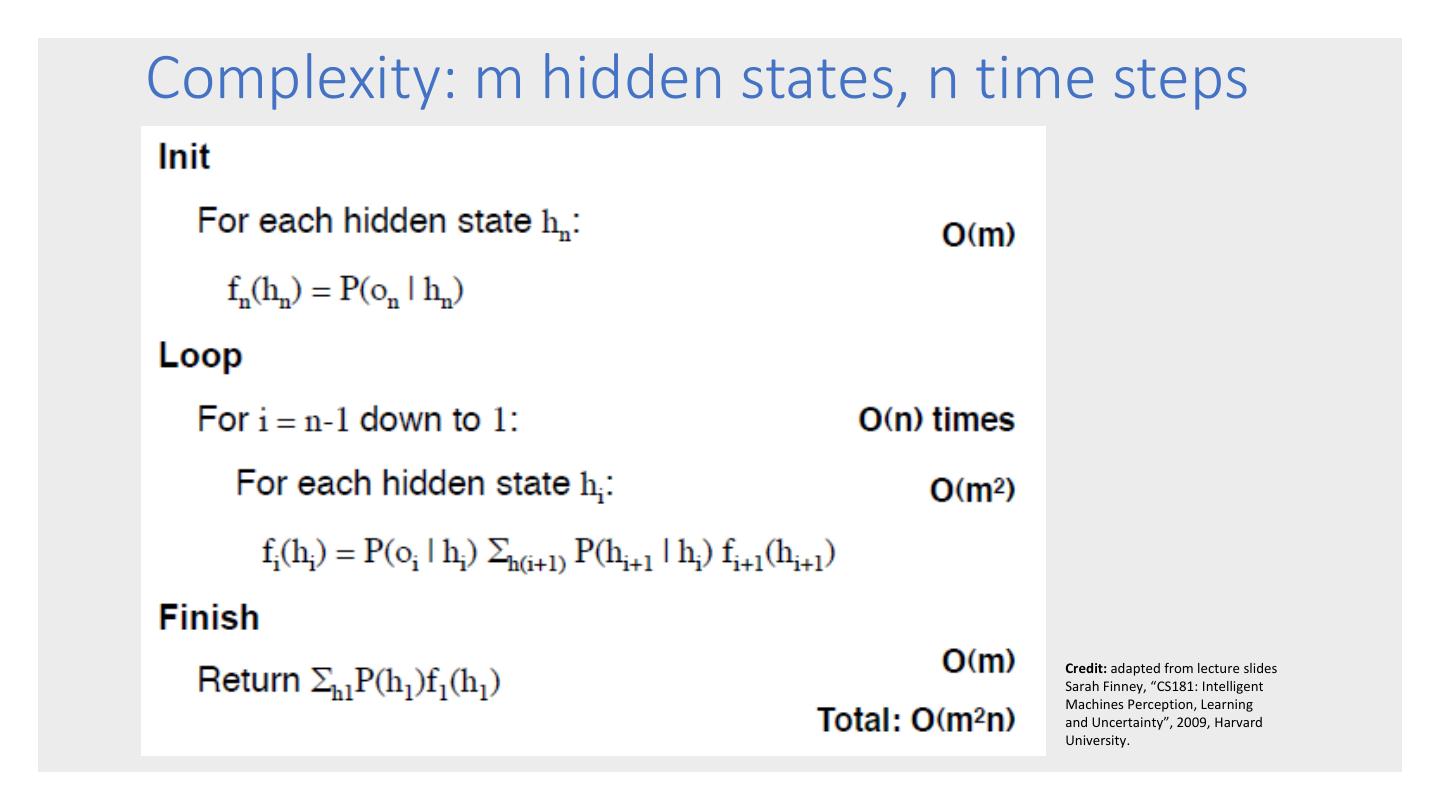
27 . • Given an HMM, the forward-backward algorithm takes as input an observation sequence 𝑜1 , … , 𝑜𝑛 , and computes 𝑃 𝑜1 , … , 𝑜𝑛 , i.e., the probability that the sequence would be generated by the HMM model. The Forward- • Uses a dynamic programming approach, which is possible because of the Markov Backward assumptions. • Relatively efficient at 𝑂 𝑚2 𝑛 where m is the Algorithm number of hidden states and n is the sequence length. • Forms the basis for sequence classification. • There are 2 forms: the forward algorithm and the backward algorithm. There is no advantage of one over the other. 

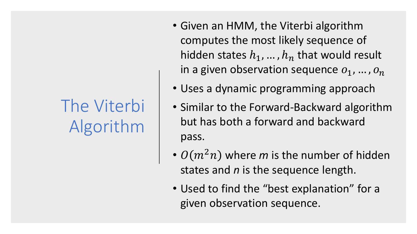
28 . • Given an HMM, the Viterbi algorithm computes the most likely sequence of hidden states ℎ1 , … , ℎ𝑛 that would result in a given observation sequence 𝑜1 , … , 𝑜𝑛 • Uses a dynamic programming approach The Viterbi • Similar to the Forward-Backward algorithm but has both a forward and backward Algorithm pass. • 𝑂 𝑚2 𝑛 where m is the number of hidden states and n is the sequence length. • Used to find the “best explanation” for a given observation sequence. 

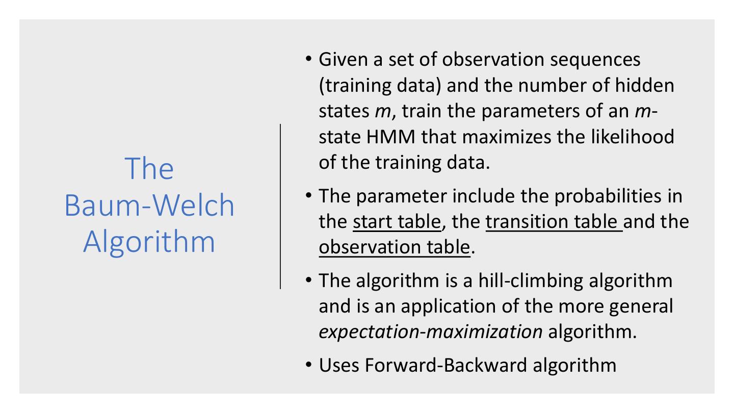
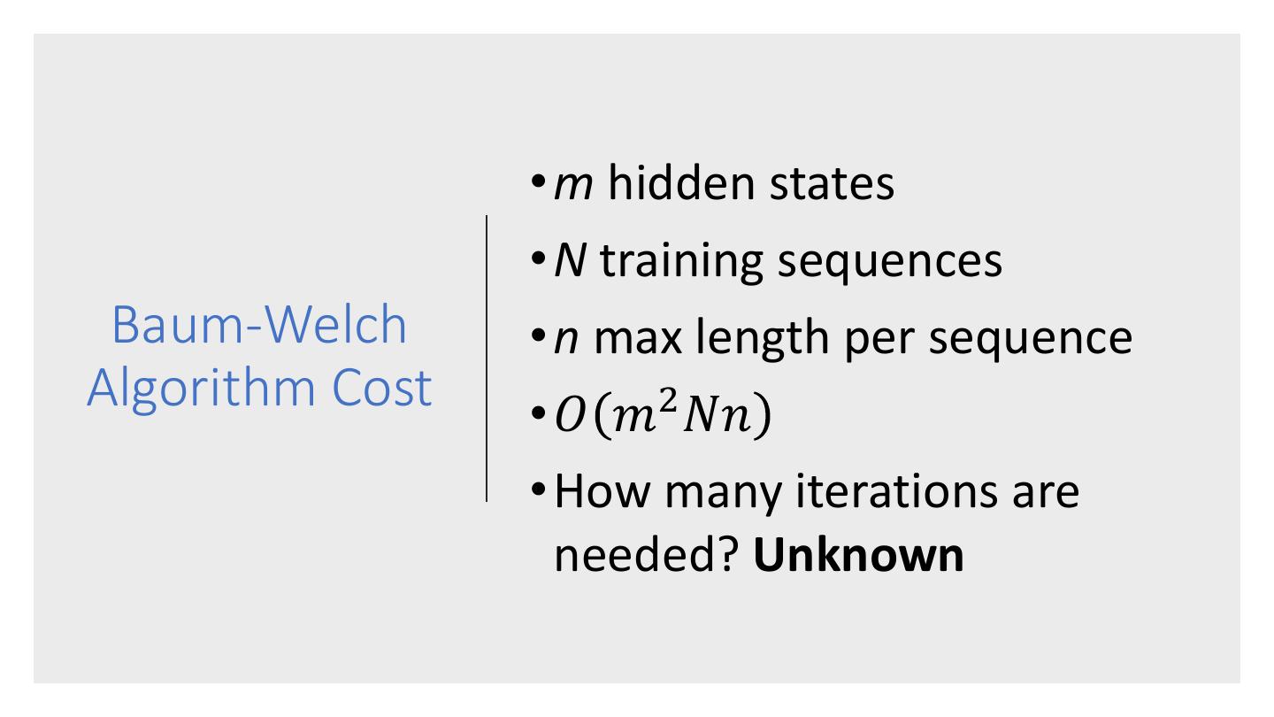
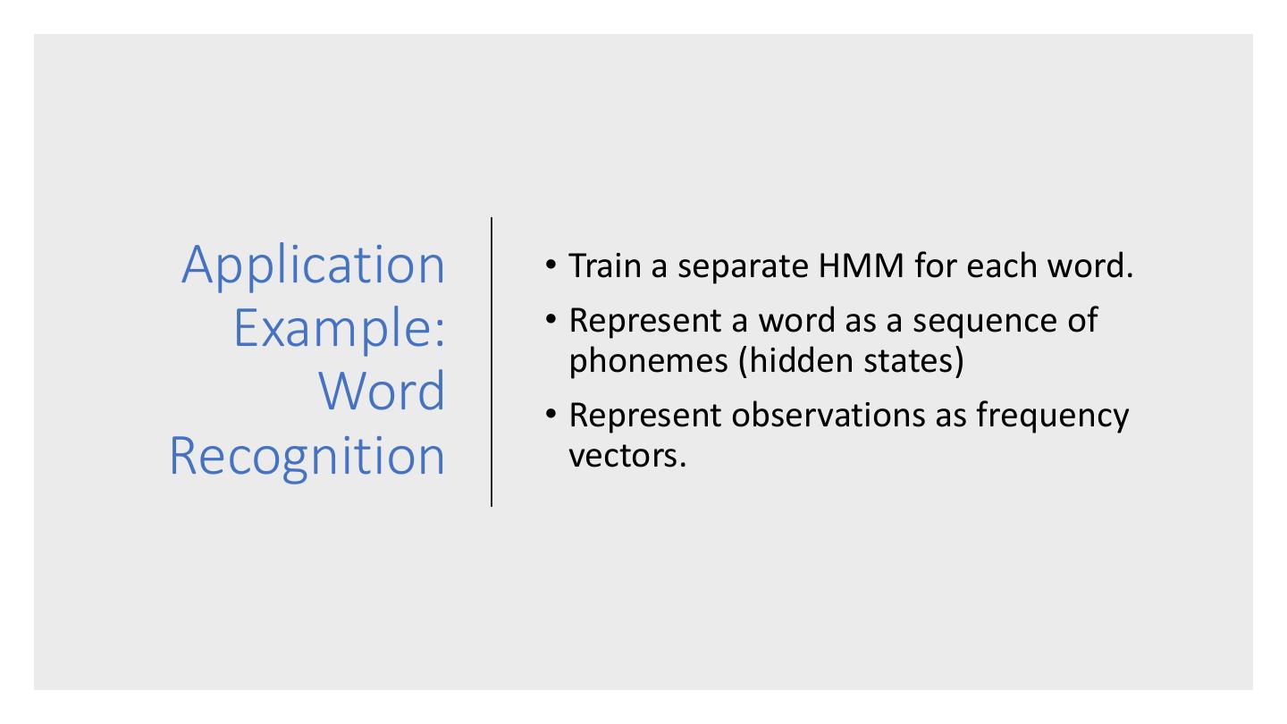
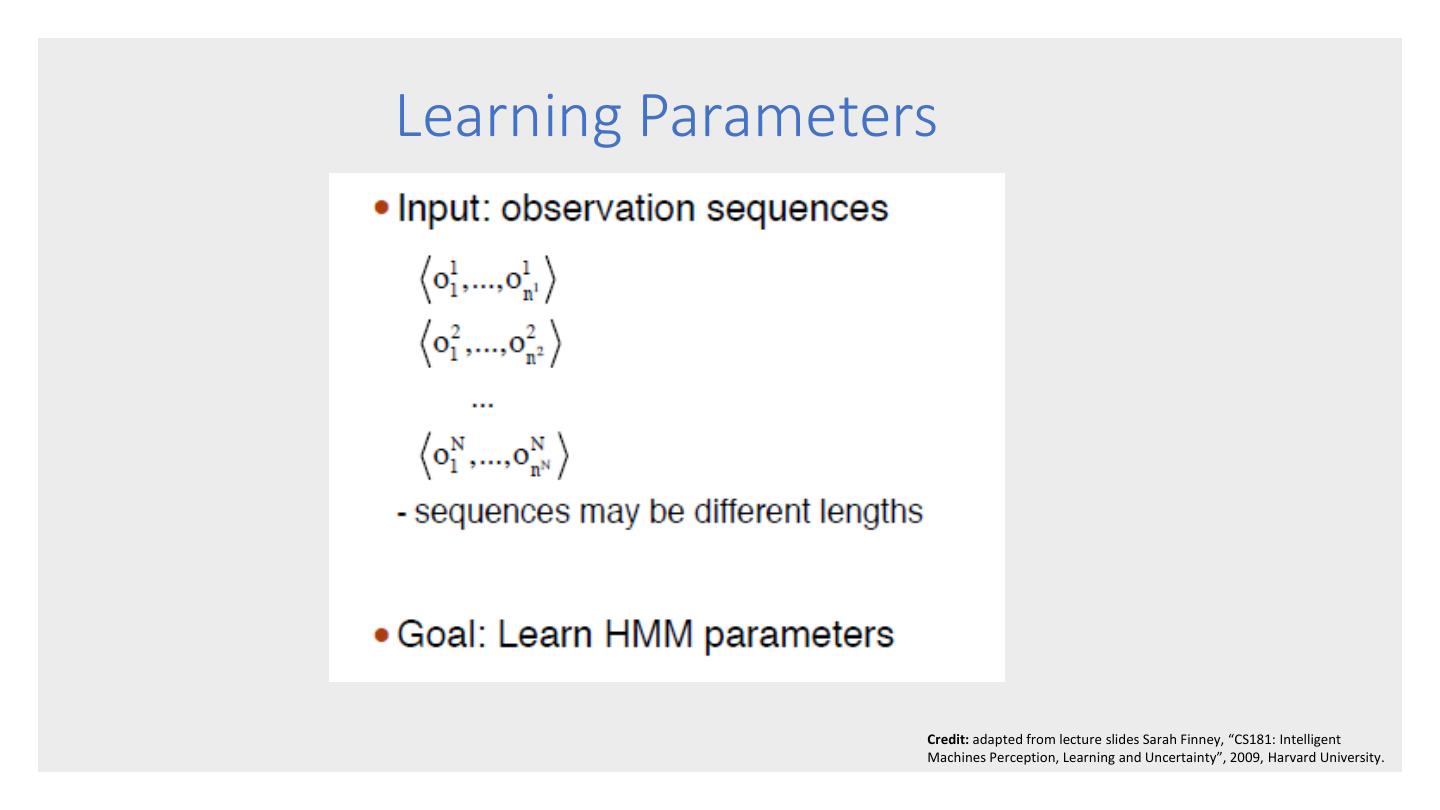
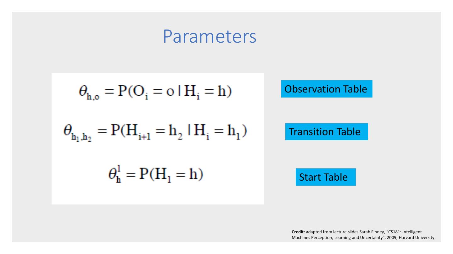
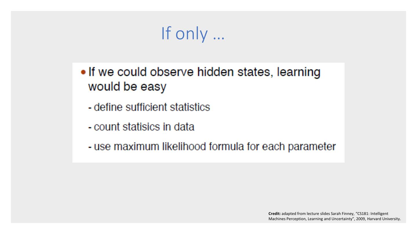
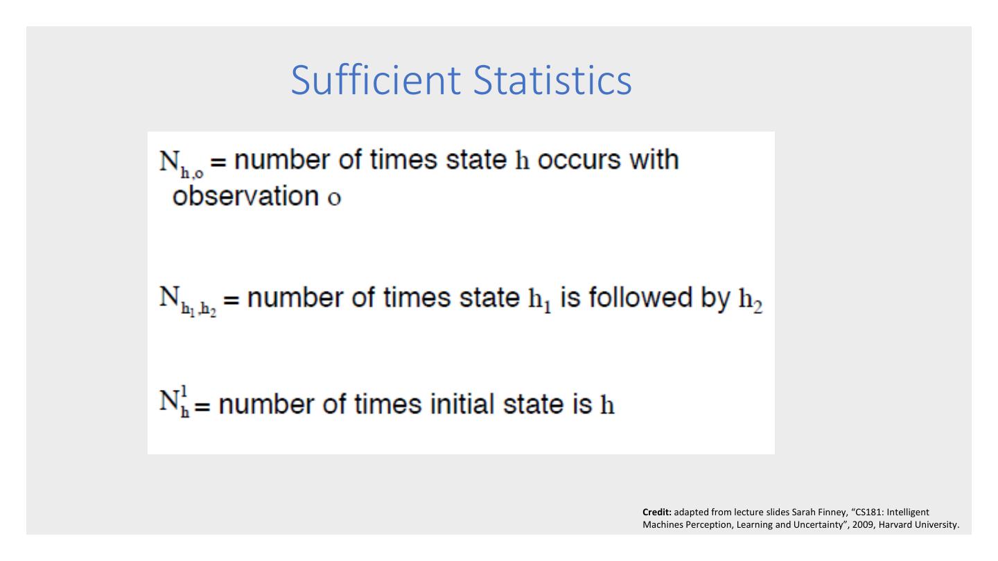
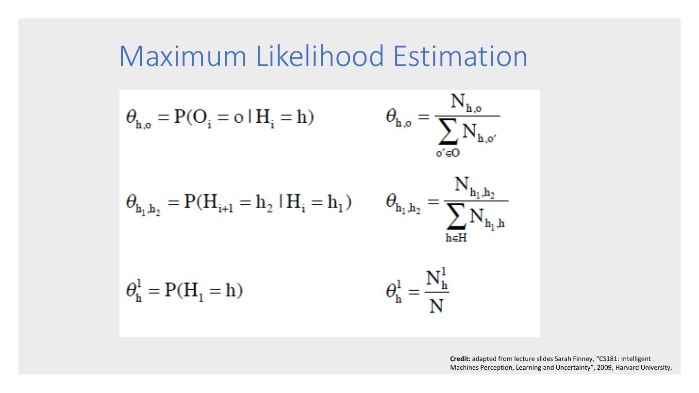
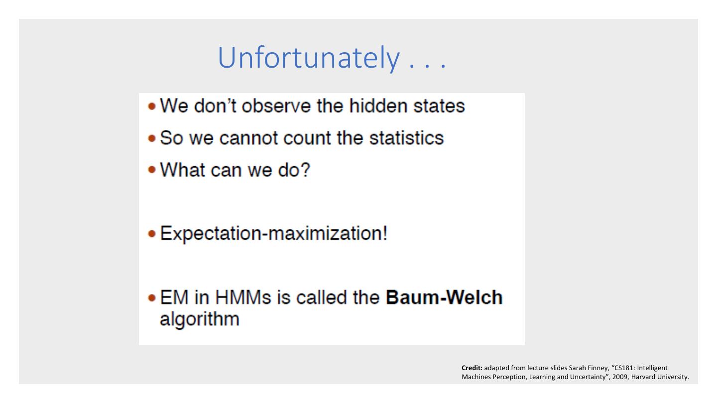
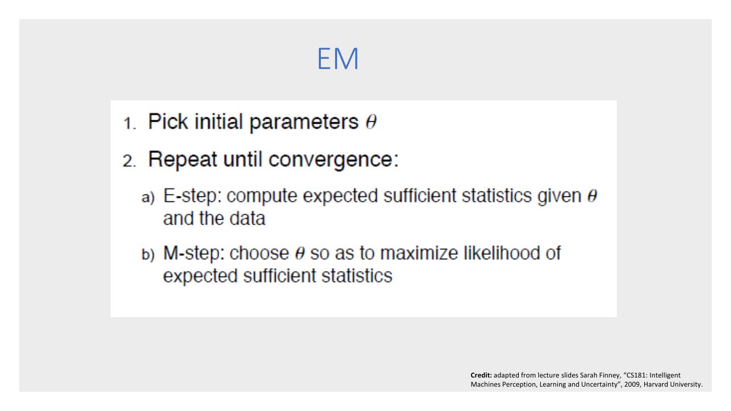
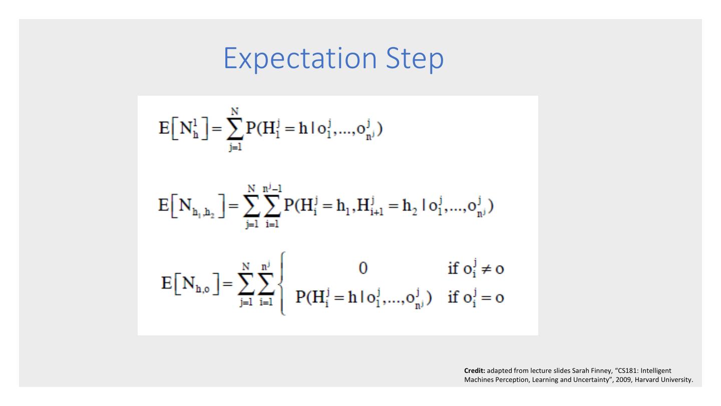
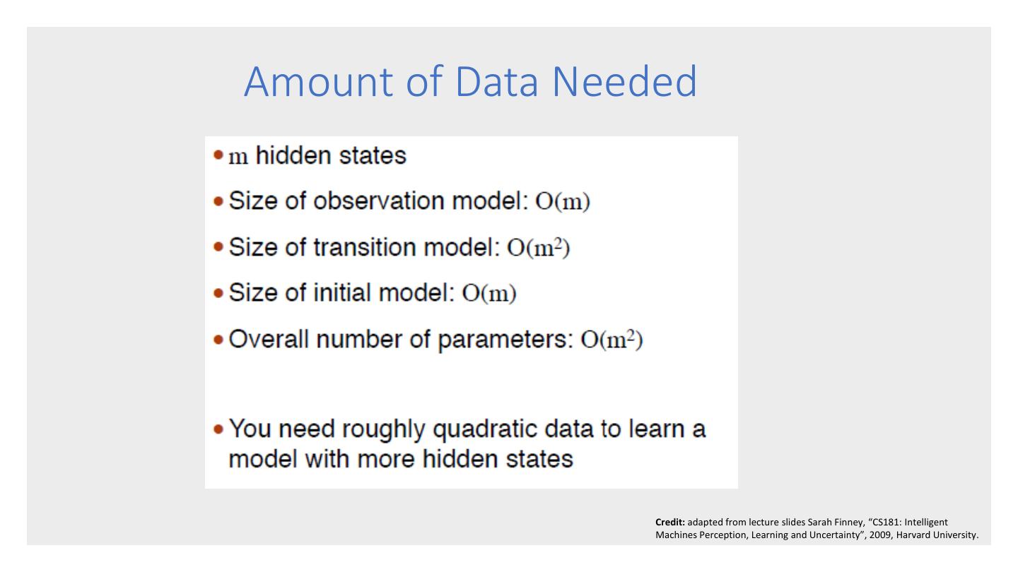
29 . • Given a set of observation sequences (training data) and the number of hidden states m, train the parameters of an m- state HMM that maximizes the likelihood The of the training data. • The parameter include the probabilities in Baum-Welch the start table, the transition table and the Algorithm observation table. • The algorithm is a hill-climbing algorithm and is an application of the more general expectation-maximization algorithm. • Uses Forward-Backward algorithm