04_Fitting_Probability_Models

1 .Computer vision: models, learning and inference Chapter 4 Fitting Probability Models

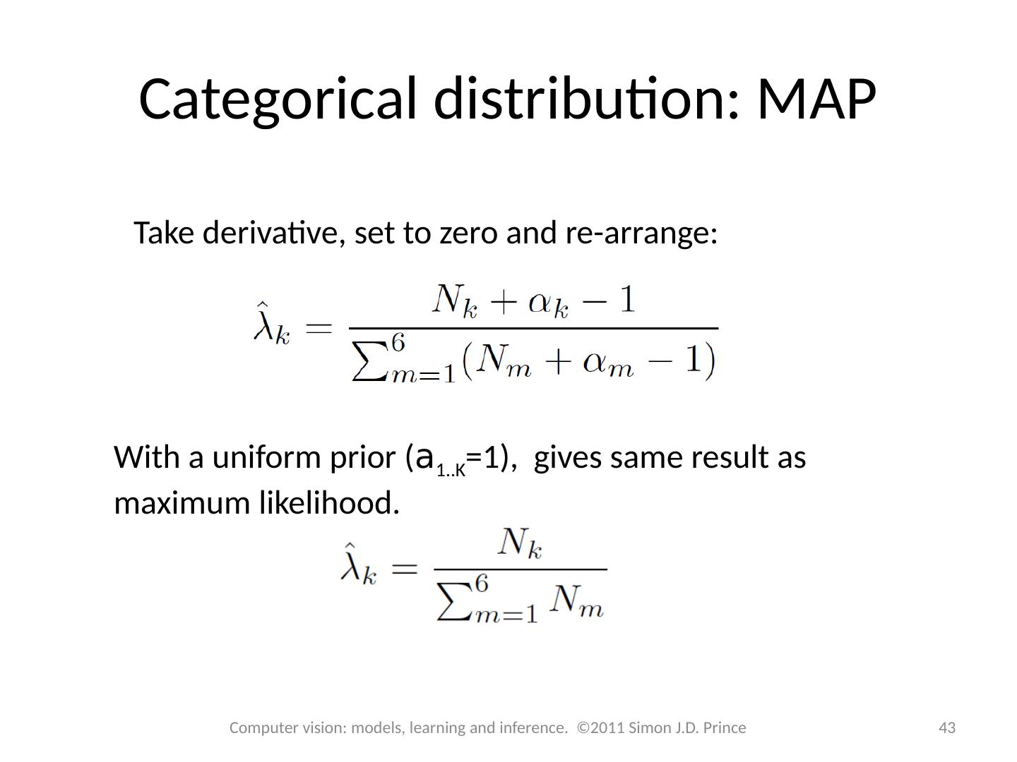
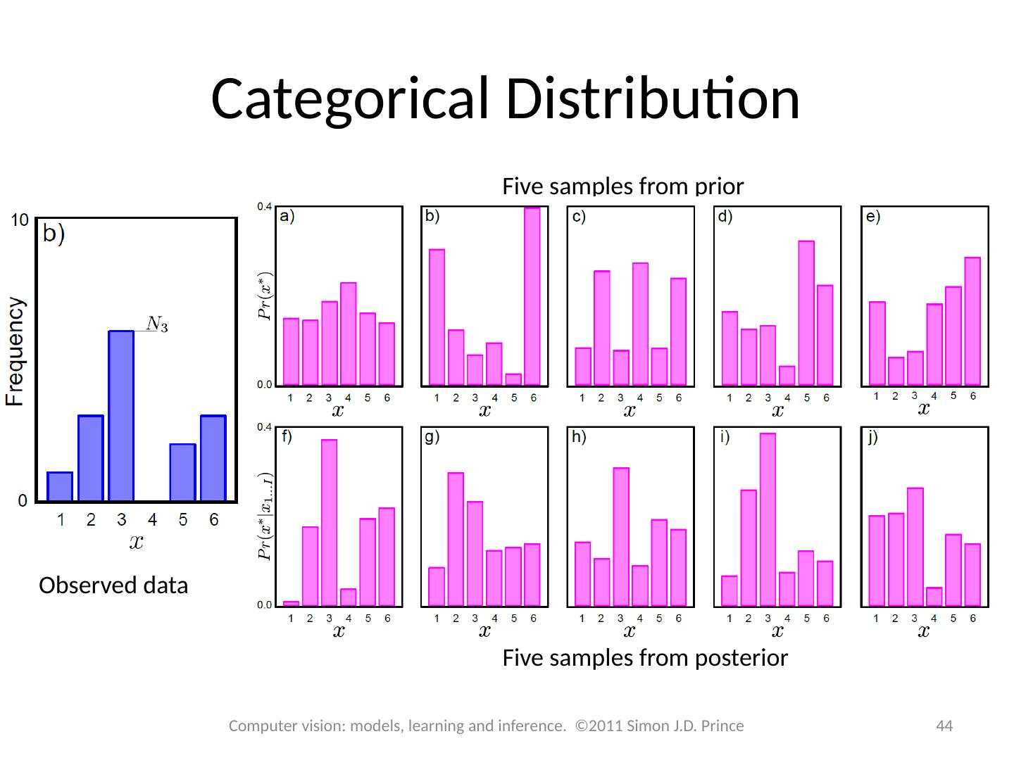
2 .Structure 2 2 Computer vision: models, learning and inference. ©2011 Simon J.D. Prince Fitting probability distributions Maximum likelihood Maximum a posteriori Bayesian approach Worked example 1: Normal distribution Worked example 2: Categorical distribution

3 .Fitting: As the name suggests: find the parameters under which the data are most likely: Maximum Likelihood 3 Computer vision: models, learning and inference. ©2011 Simon J.D. Prince Predictive Density: Evaluate new data point under probability distribution with best parameters We have assumed that data was independent (hence product)

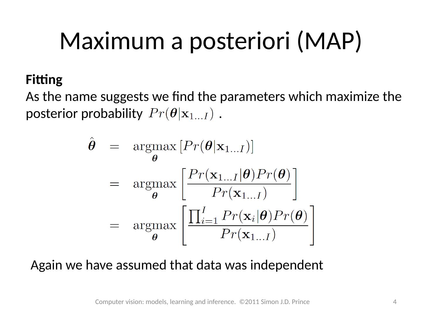
4 .Maximum a posteriori (MAP) Fitting As the name suggests we find the parameters which maximize the posterior probability . 4 Computer vision: models, learning and inference. ©2011 Simon J.D. Prince Again we have assumed that data was independent

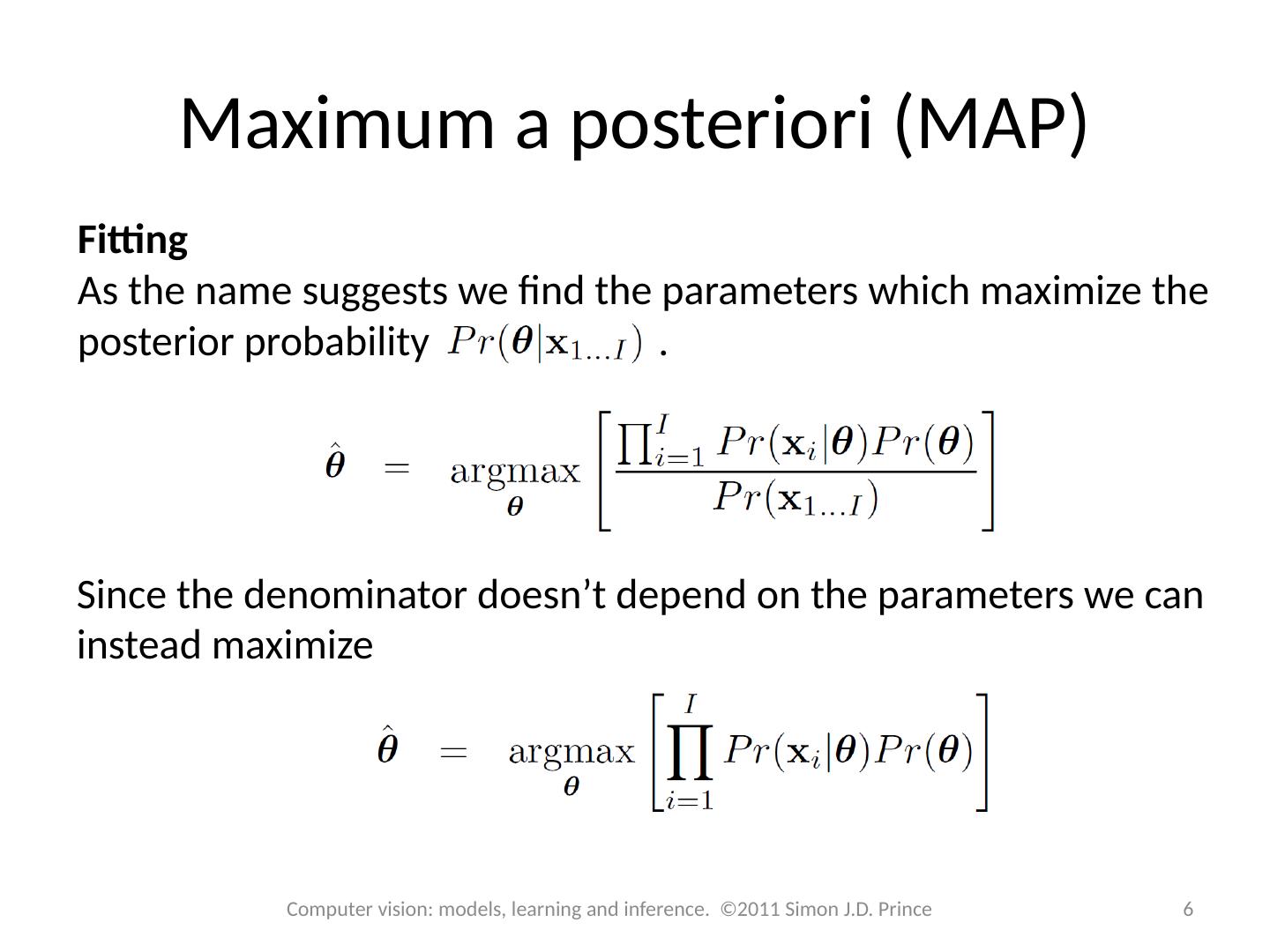
5 .Maximum a posteriori (MAP) Fitting As the name suggests we find the parameters which maximize the posterior probability . Since the denominator doesn’t depend on the parameters we can instead maximize 5 Computer vision: models, learning and inference. ©2011 Simon J.D. Prince

6 .Maximum a posteriori (MAP) Fitting As the name suggests we find the parameters which maximize the posterior probability . 6 Computer vision: models, learning and inference. ©2011 Simon J.D. Prince Since the denominator doesn’t depend on the parameters we can instead maximize

7 .Maximum a posteriori (MAP) Predictive Density: Evaluate new data point under probability distribution with MAP parameters 7 Computer vision: models, learning and inference. ©2011 Simon J.D. Prince

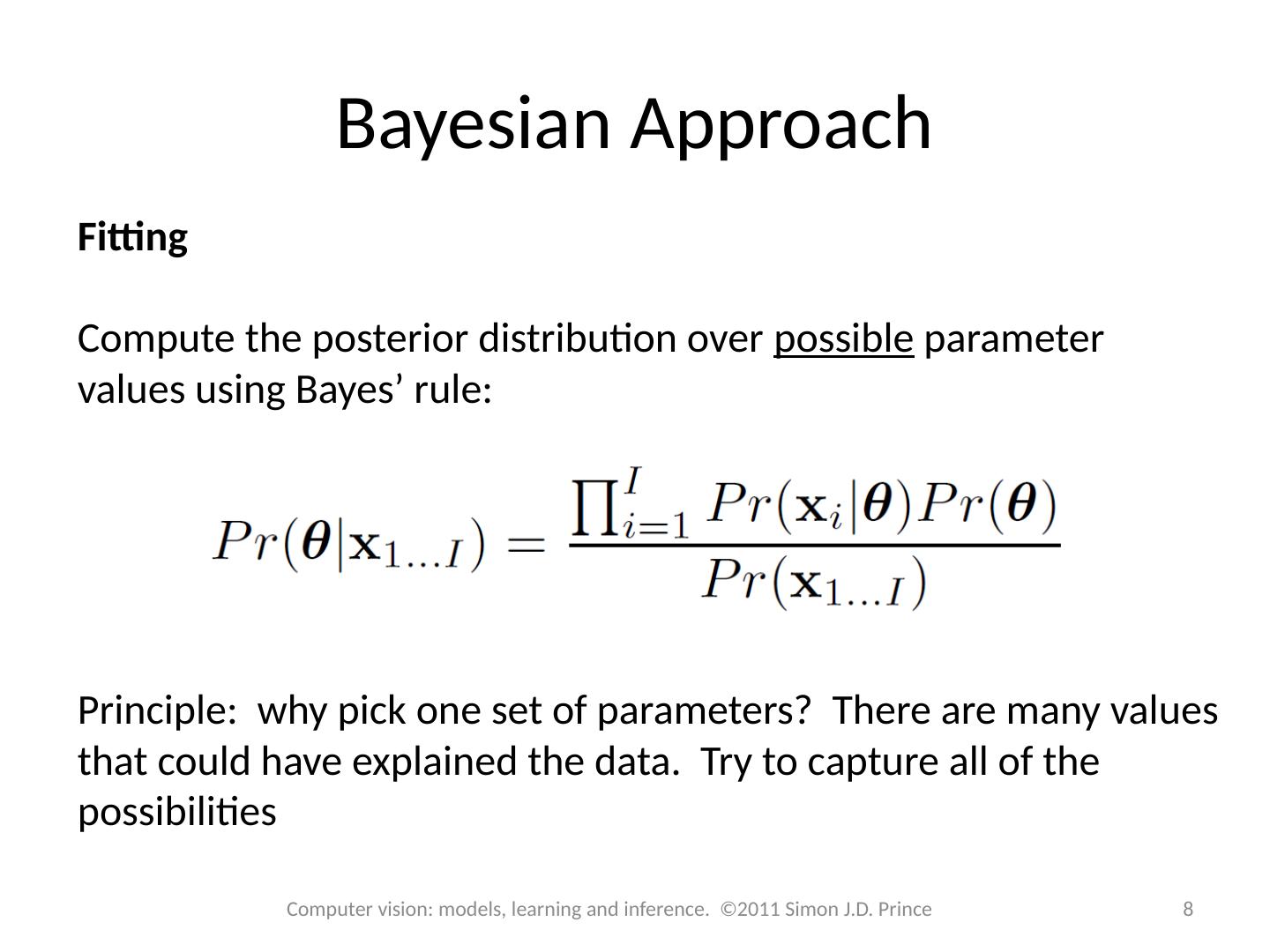
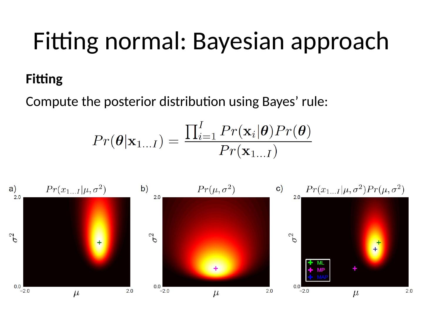
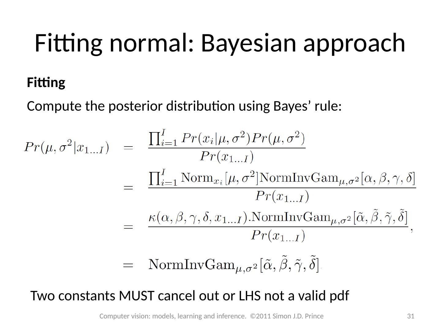
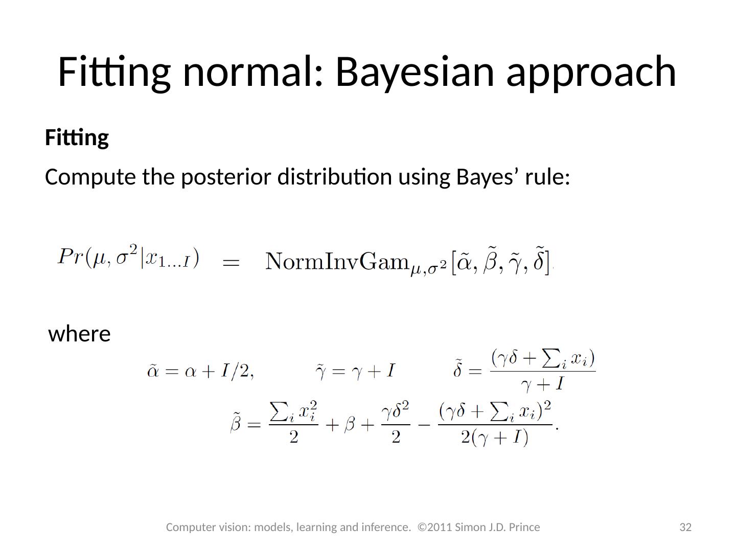
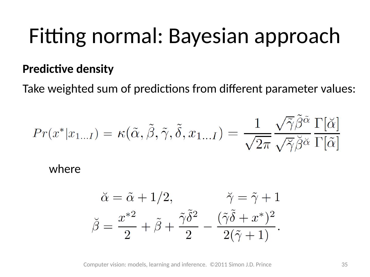
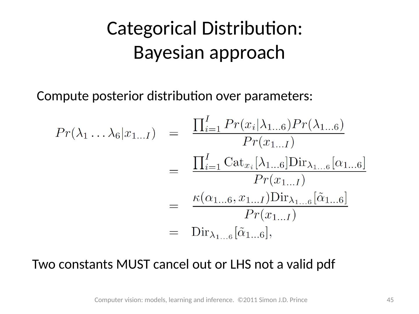
8 .Bayesian Approach Fitting Compute the posterior distribution over possible parameter values using Bayes ’ rule: Principle: why pick one set of parameters? There are many values that could have explained the data. Try to capture all of the possibilities 8 Computer vision: models, learning and inference. ©2011 Simon J.D. Prince

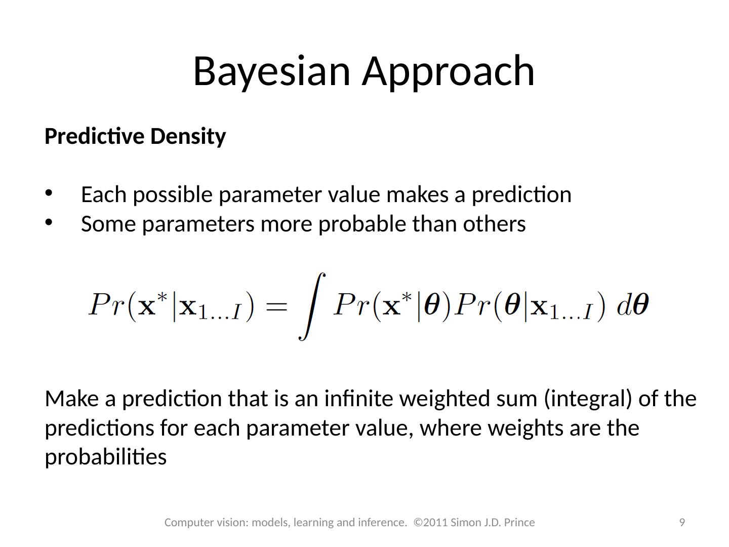
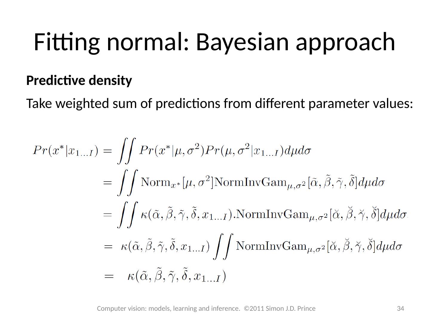
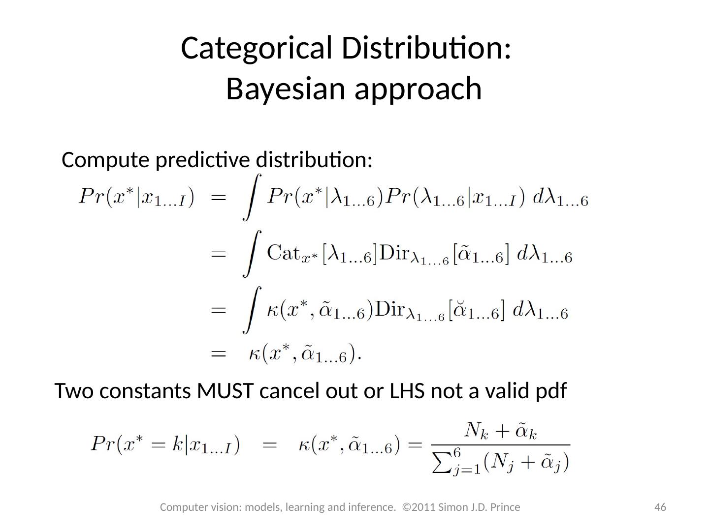
9 .Bayesian Approach Predictive Density Each possible parameter value makes a prediction Some parameters more probable than others Make a prediction that is an infinite weighted sum (integral) of the predictions for each parameter value, where weights are the probabilities 9 Computer vision: models, learning and inference. ©2011 Simon J.D. Prince

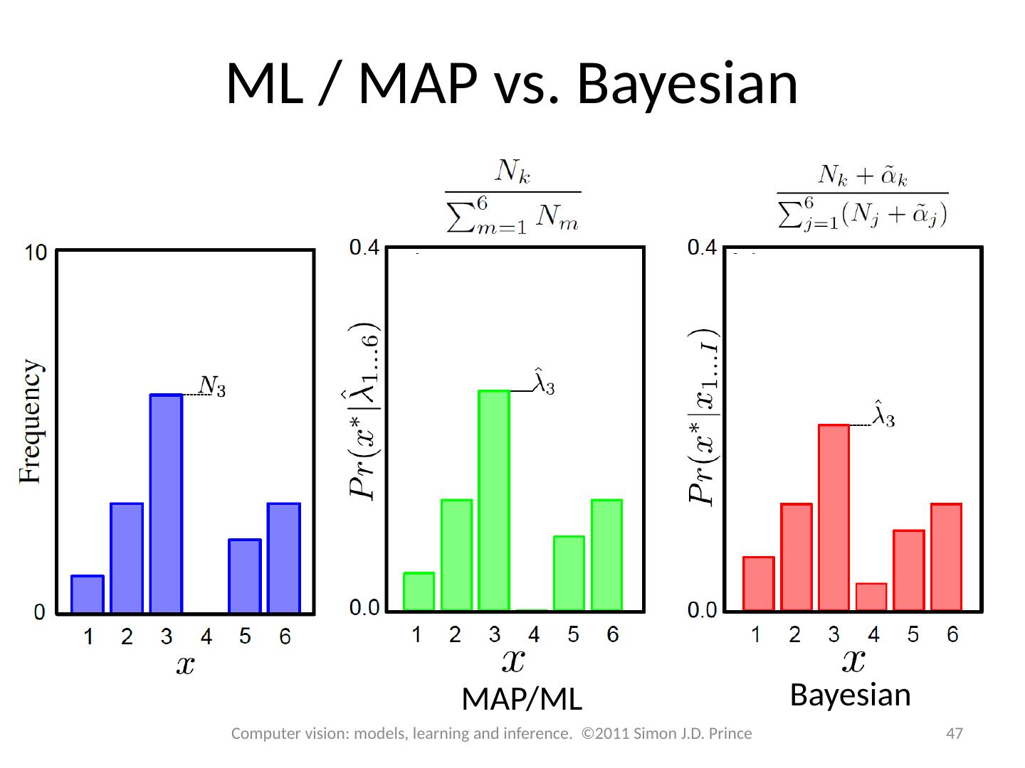
10 .Predictive densities for 3 methods Maximum a posteriori: Evaluate new data point under probability distribution with MAP parameters Maximum likelihood: Evaluate new data point under probability distribution with ML parameters Bayesian: Calculate weighted sum of predictions from all possible values of parameters 10 Computer vision: models, learning and inference. ©2011 Simon J.D. Prince

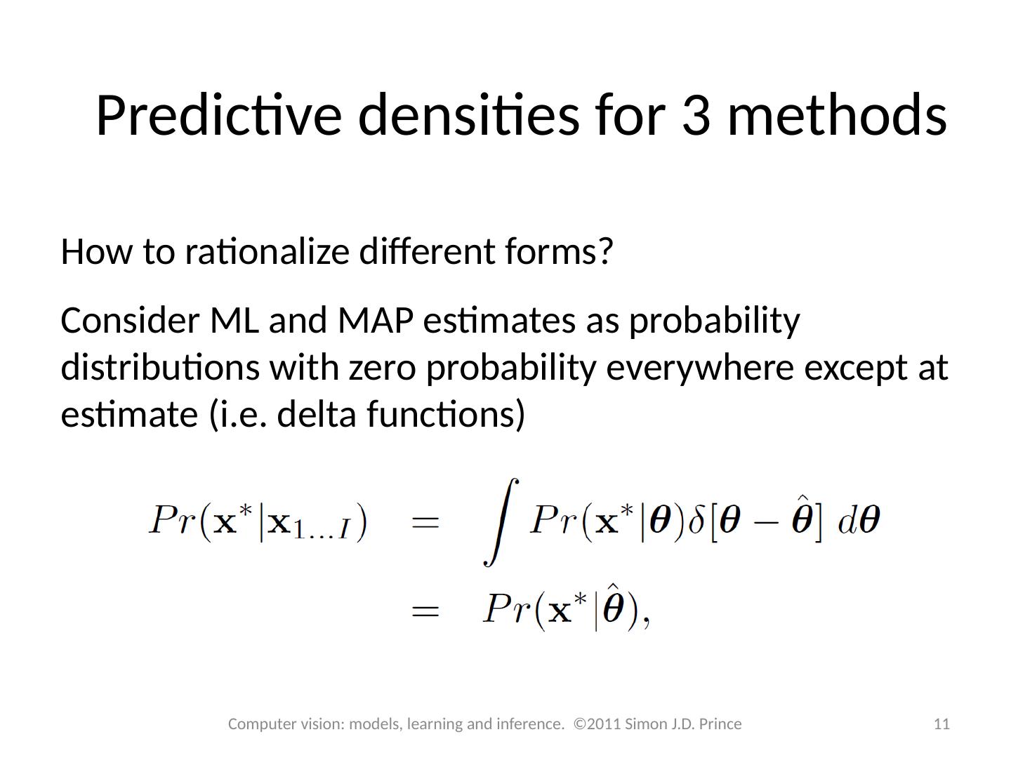
11 .How to rationalize different forms? Consider ML and MAP estimates as probability distributions with zero probability everywhere except at estimate (i.e. delta functions) Predictive densities for 3 methods 11 Computer vision: models, learning and inference. ©2011 Simon J.D. Prince

12 .Structure 12 12 Computer vision: models, learning and inference. ©2011 Simon J.D. Prince Fitting probability distributions Maximum likelihood Maximum a posteriori Bayesian approach Worked example 1: Normal distribution Worked example 2: Categorical distribution

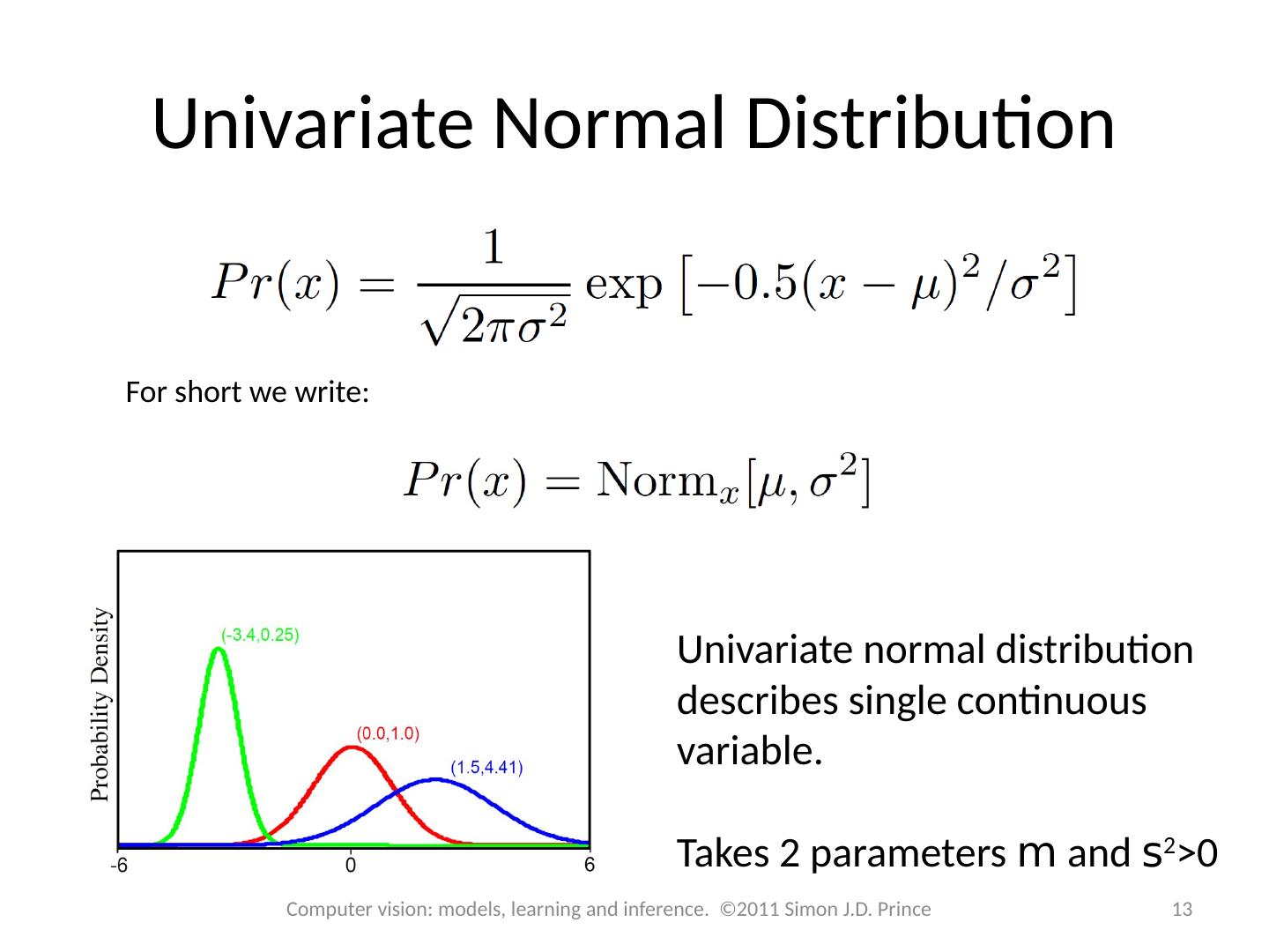
13 .Univariate Normal Distribution For short we write: Univariate normal distribution describes single continuous variable. Takes 2 parameters m and s 2 >0 13 Computer vision: models, learning and inference. ©2011 Simon J.D. Prince

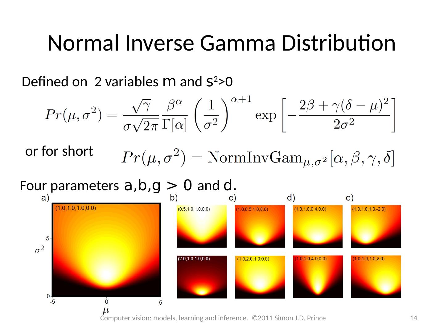
14 .Normal Inverse Gamma Distribution Defined on 2 variables m and s 2 >0 o r for short Four parameters a,b,g > 0 and d. 14 Computer vision: models, learning and inference. ©2011 Simon J.D. Prince

15 .Ready? Approach the same problem 3 different ways: Learn ML parameters Learn MAP parameters Learn Bayesian distribution of parameters Will we get the same results? 15 Computer vision: models, learning and inference. ©2011 Simon J.D. Prince

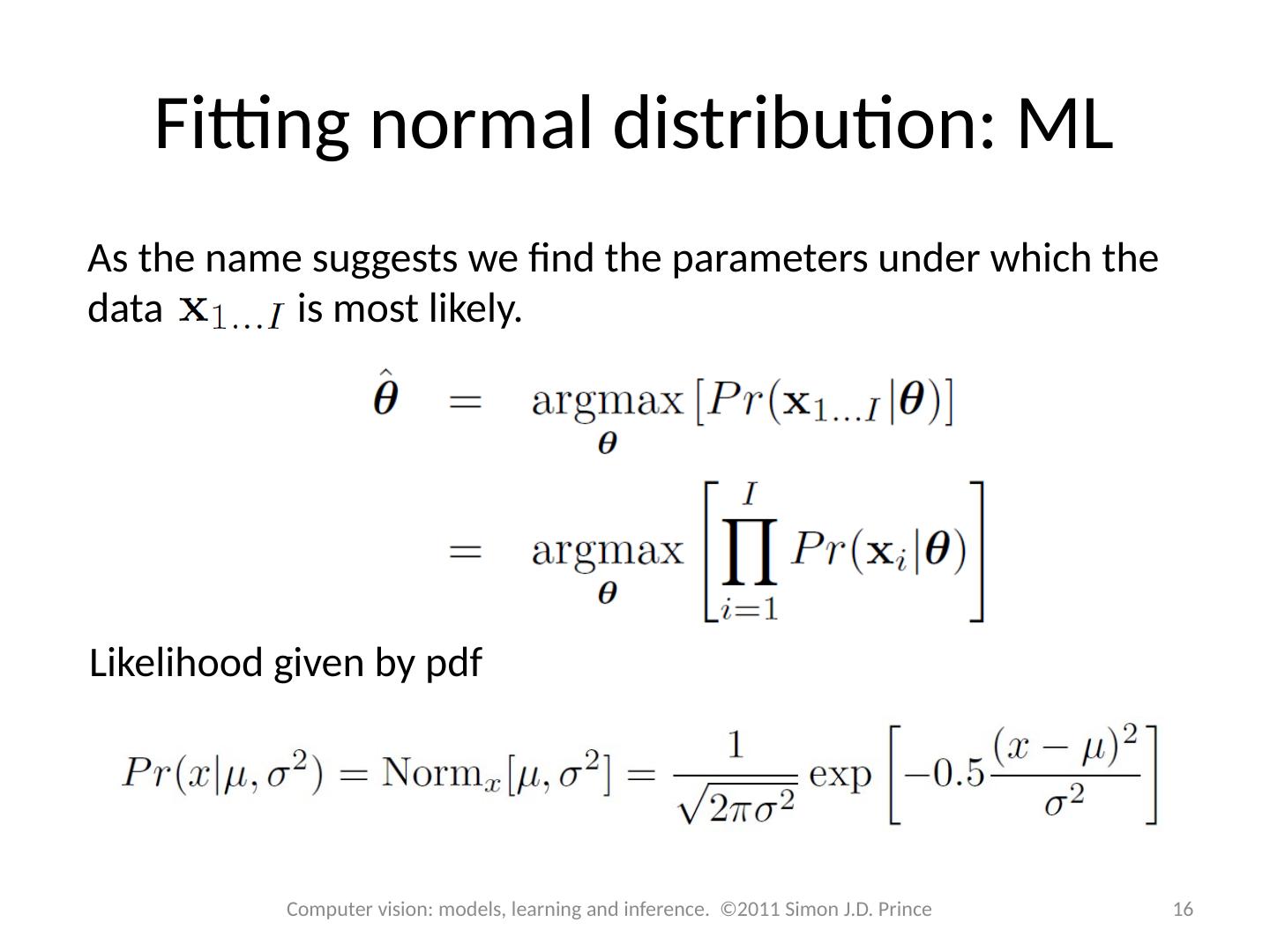
16 .As the name suggests we find the parameters under which the data is most likely. Fitting normal distribution: ML 16 Computer vision: models, learning and inference. ©2011 Simon J.D. Prince Likelihood given by pdf

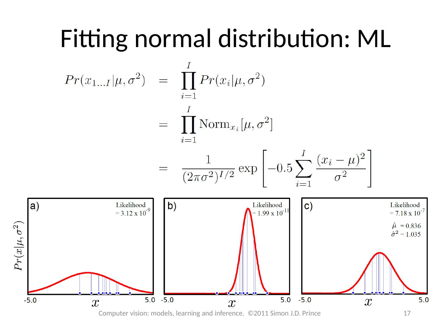
17 .Fitting normal distribution: ML 17 Computer vision: models, learning and inference. ©2011 Simon J.D. Prince

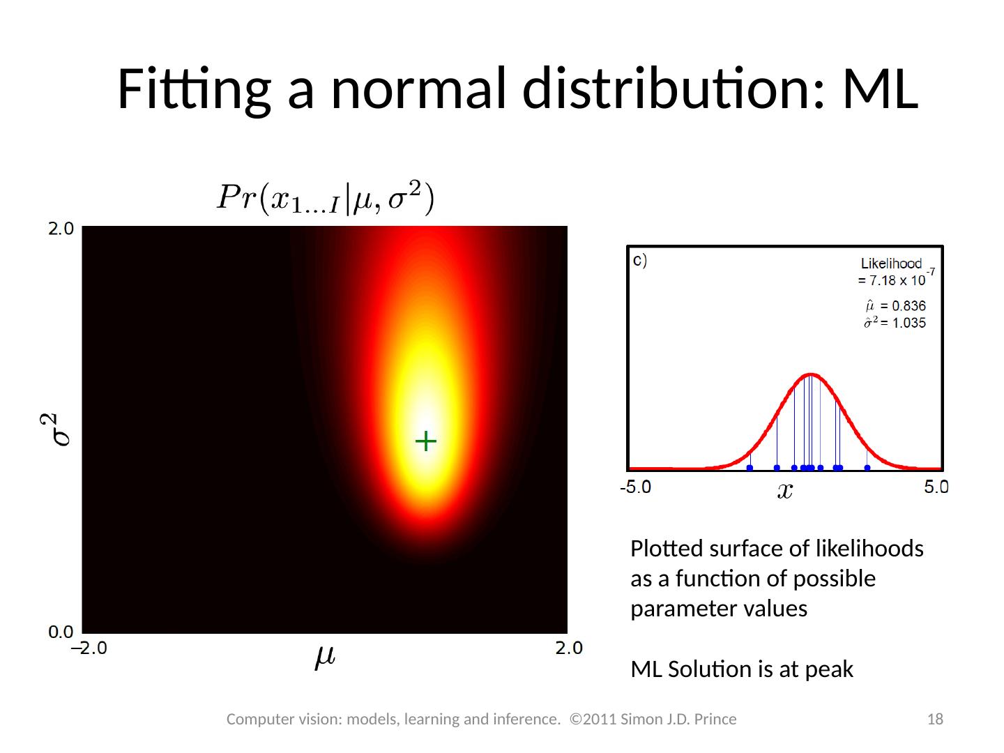
18 .Fitting a normal distribution: ML Plotted surface of likelihoods as a function of possible parameter values ML Solution is at peak 18 Computer vision: models, learning and inference. ©2011 Simon J.D. Prince

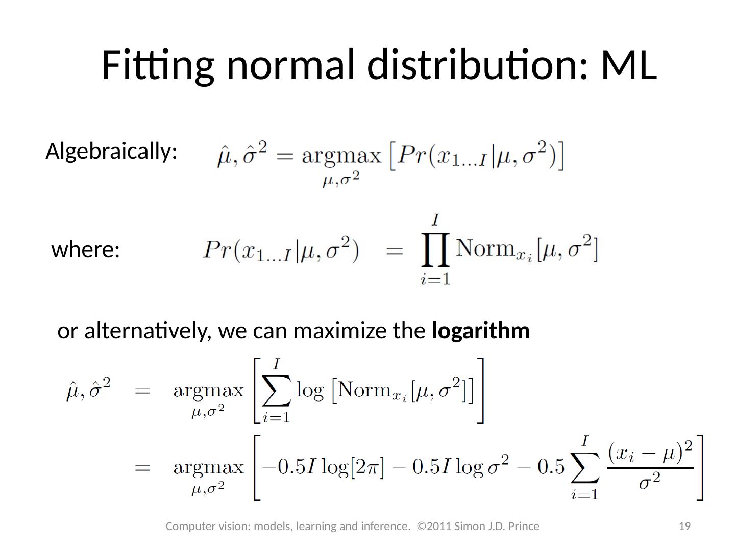
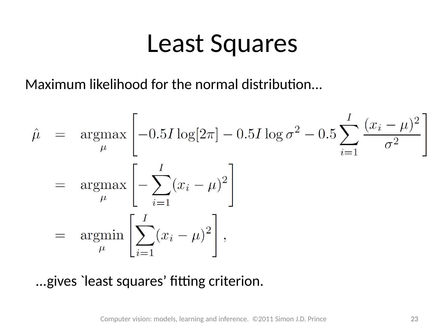
19 .Fitting normal distribution: ML Algebraically: or alternatively, we can maximize the logarithm 19 Computer vision: models, learning and inference. ©2011 Simon J.D. Prince where:

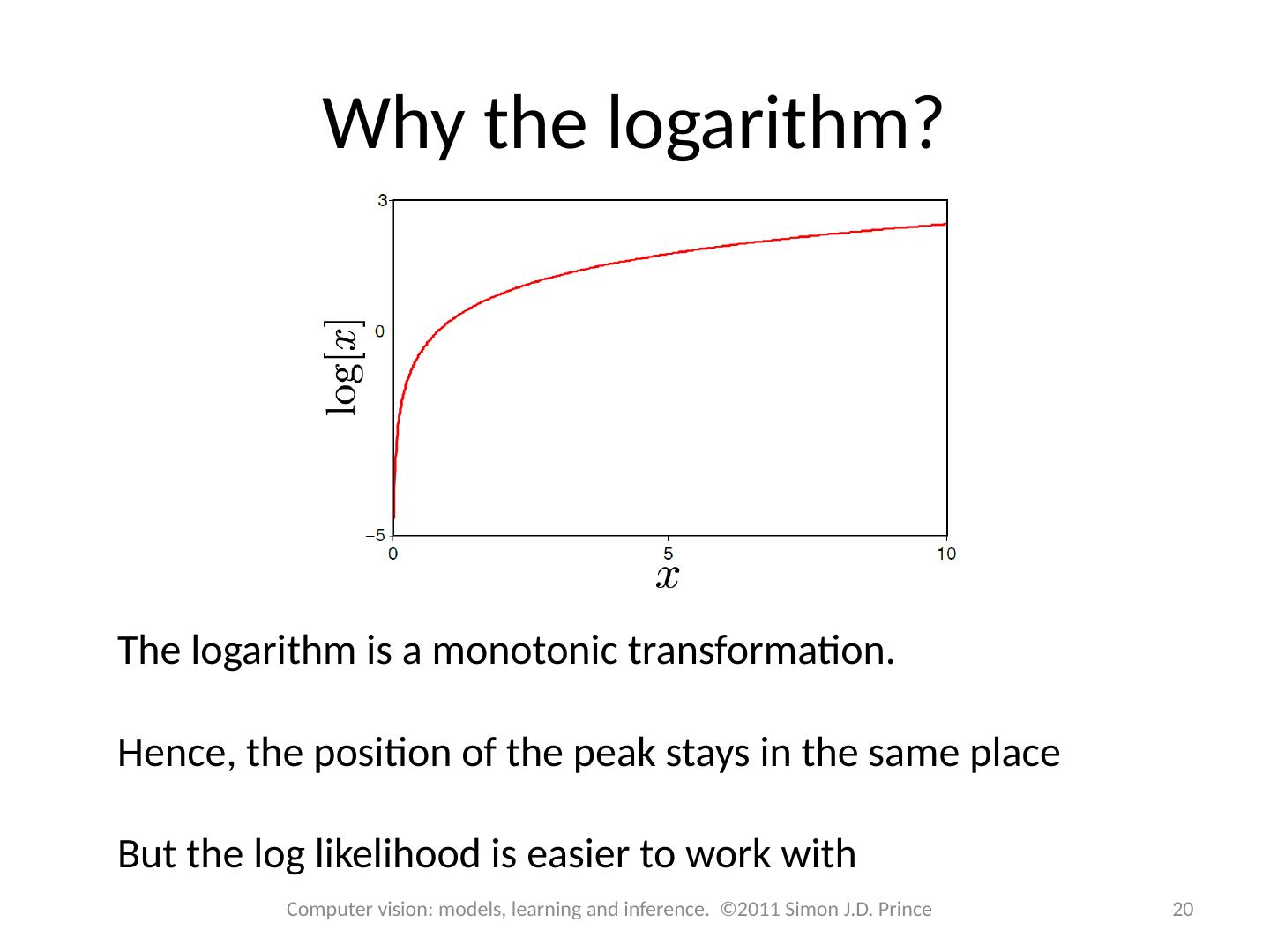
20 .Why the logarithm? The logarithm is a monotonic transformation. Hence, the position of the peak stays in the same place But the log likelihood is easier to work with 20 Computer vision: models, learning and inference. ©2011 Simon J.D. Prince

21 .Fitting normal distribution: ML How to maximize a function? Take derivative and equate to zero. 21 Computer vision: models, learning and inference. ©2011 Simon J.D. Prince Solution:

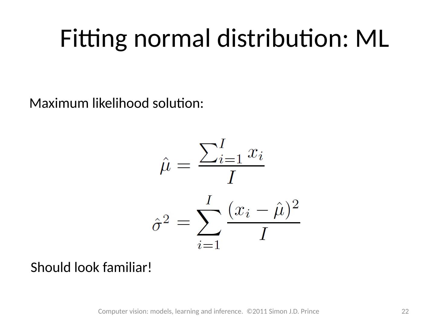
22 .Fitting normal distribution: ML Maximum likelihood solution: Should look familiar! 22 Computer vision: models, learning and inference. ©2011 Simon J.D. Prince

23 .Computer vision: models, learning and inference. ©2011 Simon J.D. Prince Least Squares 23 23 Maximum likelihood for the normal distribution... ...gives `least squares’ fitting criterion.

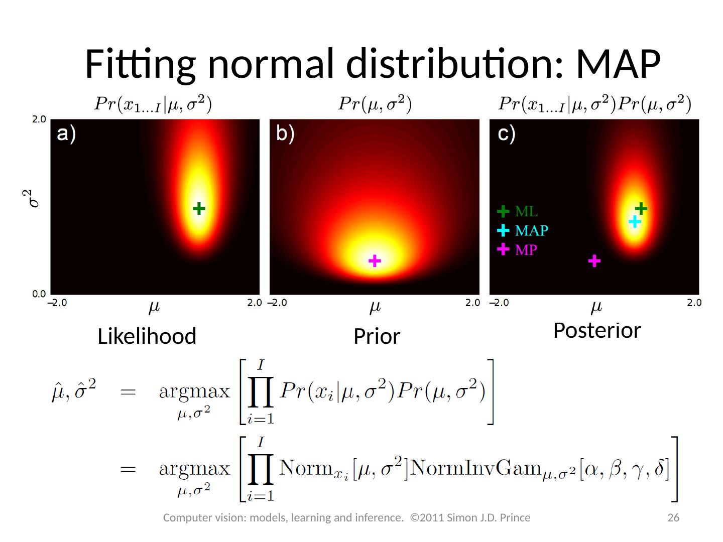
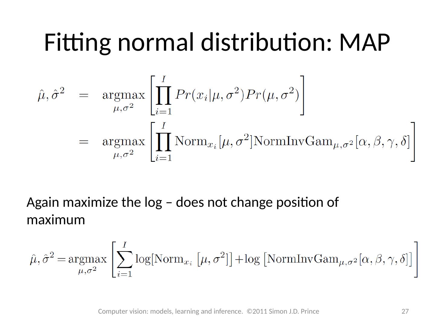
24 .Fitting normal distribution: MAP Fitting As the name suggests we find the parameters which maximize the posterior probability .. Likelihood is normal PDF 24 Computer vision: models, learning and inference. ©2011 Simon J.D. Prince

25 .Fitting normal distribution: MAP Prior Use conjugate prior, normal scaled inverse gamma. 25 Computer vision: models, learning and inference. ©2011 Simon J.D. Prince

26 .Fitting normal distribution: MAP Likelihood Prior Posterior 26 Computer vision: models, learning and inference. ©2011 Simon J.D. Prince

27 .Fitting normal distribution: MAP Again maximize the log – does not change position of maximum 27 Computer vision: models, learning and inference. ©2011 Simon J.D. Prince

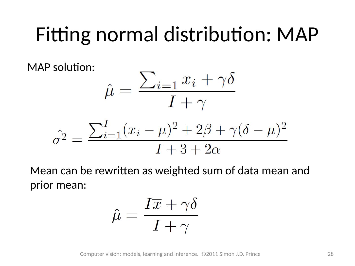
28 .Fitting normal distribution: MAP MAP solution: Mean can be rewritten as weighted sum of data mean and prior mean: 28 Computer vision: models, learning and inference. ©2011 Simon J.D. Prince

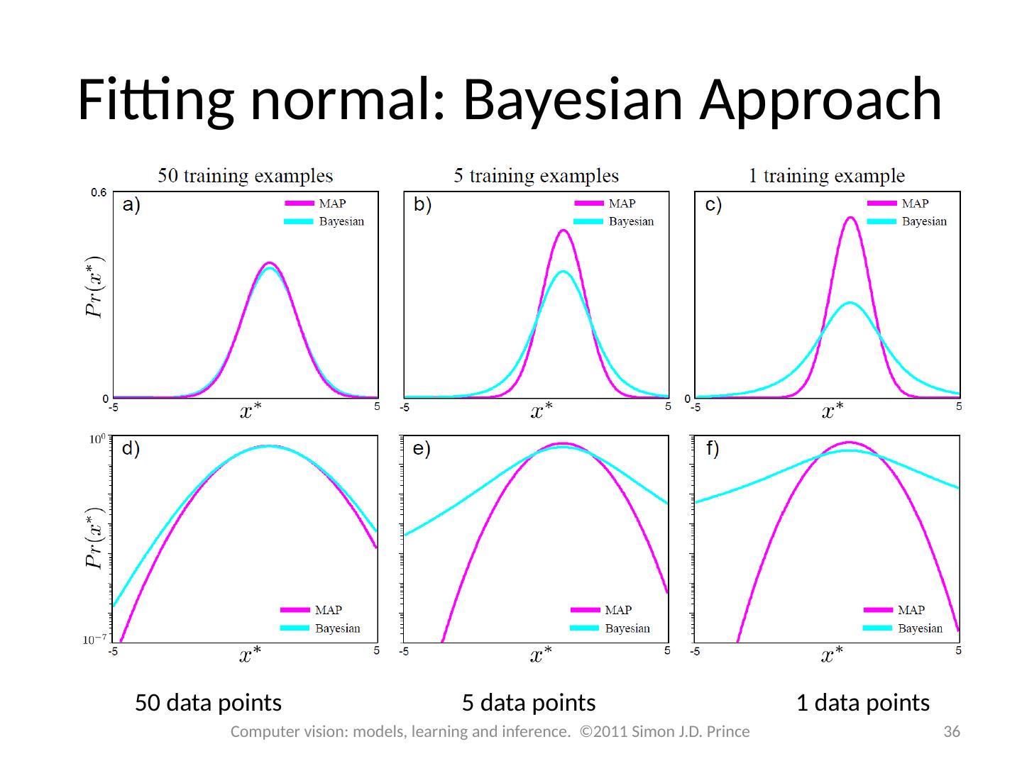
29 .Fitting normal distribution: MAP 50 data points 5 data points 1 data points