prototype methods:K-means

1 .Prototype Methods: K-Means Prototype Methods: K-Means Jia Li Department of Statistics The Pennsylvania State University Email: jiali@stat.psu.edu http://www.stat.psu.edu/∼jiali Jia Li http://www.stat.psu.edu/∼jiali 

2 .Prototype Methods: K-Means Prototype Methods Essentially model-free. Not useful for understanding the nature of the relationship between the features and class outcome. They can be very effective as black box prediction engines. Training data: {(x1 , g1 ), (x2 , g2 ), ..., (xN , gN )}. The class labels gi ∈ {1, 2, ..., K }. Represent the training data by a set of points in feature space, also called prototypes. Each prototype has an associated class label, and classification of a query point x is made to the class of the closest prototype. Methods differ according to how the number and the positions of the prototypes are decided. Jia Li http://www.stat.psu.edu/∼jiali 

3 .Prototype Methods: K-Means K-means Assume there are M prototypes denoted by Z = {z1 , z2 , ..., zM } . Each training sample is assigned to one of the prototype. Denote the assignment function by A(·). Then A(xi ) = j means the ith training sample is assigned to the jth prototype. Goal: minimize the total mean squared error between the training samples and their representative prototypes, that is, the trace of the pooled within cluster covariance matrix. N 2 arg min xi − zA(xi ) Z,A i=1 Jia Li http://www.stat.psu.edu/∼jiali 

4 .Prototype Methods: K-Means Denote the objective function by N 2 L(Z, A) = xi − zA(xi ) . i=1 Intuition: training samples are tightly clustered around the prototypes. Hence, the prototypes serve as a compact representation for the training data. Jia Li http://www.stat.psu.edu/∼jiali 

5 .Prototype Methods: K-Means Necessary Conditions If Z is fixed, the optimal assignment function A(·) should follow the nearest neighbor rule, that is, A(xi ) = arg minj∈{1,2,...,M} xi − zj . If A(·) is fixed, the prototype zj should be the average (centroid) of all the samples assigned to the jth prototype: i:A(xi )=j xi zj = , Nj where Nj is the number of samples assigned to prototype j. Jia Li http://www.stat.psu.edu/∼jiali 

6 .Prototype Methods: K-Means The Algorithm Based on the necessary conditions, the k-means algorithm alternates the two steps: For a fixed set of centroids (prototypes), optimize A(·) by assigning each sample to its closest centroid using Euclidean distance. Update the centroids by computing the average of all the samples assigned to it. The algorithm converges since after each iteration, the objective function decreases (non-increasing). Usually converges fast. Stopping criterion: the ratio between the decrease and the objective function is below a threshold. Jia Li http://www.stat.psu.edu/∼jiali 

7 .Prototype Methods: K-Means Example Training set: {1.2, 5.6, 3.7, 0.6, 0.1, 2.6}. Apply k-means algorithm with 2 centroids, {z1 , z2 }. Initialization: randomly pick z1 = 2, z2 = 5. fixed update 2 {1.2, 0.6, 0.1, 2.6} 5 {5.6, 3.7} {1.2, 0.6, 0.1, 2.6} 1.125 {5.6, 3.7} 4.65 1.125 {1.2, 0.6, 0.1, 2.6} 4.65 {5.6, 3.7} The two prototypes are: z1 = 1.125, z2 = 4.65. The objective function is L(Z, A) = 5.3125. Jia Li http://www.stat.psu.edu/∼jiali 

8 .Prototype Methods: K-Means Initialization: randomly pick z1 = 0.8, z2 = 3.8. fixed update 0.8 {1.2, 0.6, 0.1} 3.8 {5.6, 3.7, 2.6} {1.2, 0.6, 0.1 } 0.633 {5.6, 3.7, 2.6 } 3.967 0.633 {1.2, 0.6, 0.1} 3.967 {5.6, 3.7, 2.6} The two prototypes are: z1 = 0.633, z2 = 3.967. The objective function is L(Z, A) = 5.2133. Starting from different initial values, the k-means algorithm converges to different local optimum. It can be shown that {z1 = 0.633, z2 = 3.967} is the global optimal solution. Jia Li http://www.stat.psu.edu/∼jiali 

9 .Prototype Methods: K-Means Classification by K-means The primary application of k-means is in clustering, or unsupervised classification. It can be adapted to supervised classification. Apply k-means clustering to the training data in each class separately, using R prototypes per class. Assign a class label to each of the K × R prototypes. Classify a new feature x to the class of the closest prototype. The above approach to using k-means for classification is referred to as Scheme 1. Jia Li http://www.stat.psu.edu/∼jiali 

10 .Prototype Methods: K-Means Jia Li http://www.stat.psu.edu/∼jiali 

11 .Prototype Methods: K-Means Another Approach Another approach to classification by k-means Apply k-means clustering to the entire training data, using M prototypes. For each prototype, count the number of samples from each class that are assigned to this prototype. Associate the prototype with the class that has the highest count. Classify a new feature x to the class of the closest prototype. This alternative approach is referred to as Scheme 2. Jia Li http://www.stat.psu.edu/∼jiali 

12 .Prototype Methods: K-Means Simulation Two classes both follow normal distribution with common covariance matrix. 1 0 The common covariance matrix Σ = . 0 1 The means of the two classes are: 0.0 1.5 µ1 = µ2 = 0.0 1.5 The prior probabilities of the two classes are π1 = 0.3, π2 = 0.7. A training and a testing data set are generated, each with 2000 samples. Jia Li http://www.stat.psu.edu/∼jiali 

13 .Prototype Methods: K-Means The optimal decision boundary between the two classes is given by LDA, since the two class-conditioned densities of the input are both normal with common covariance matrix. The optimal decision rule is (i.e., the Bayes rule): 1 X1 + X2 ≤ 0.9351 G (X ) = 2 otherwise The error rate computed using the test data set and the optimal decision rule is 11.75%. Jia Li http://www.stat.psu.edu/∼jiali 

14 .Prototype Methods: K-Means The scatter plot of the training data set. Red star: Class 1. Blue circle: Class 2. Jia Li http://www.stat.psu.edu/∼jiali 

15 .Prototype Methods: K-Means K-means with Scheme 1 For each class, use R = 6 prototypes. The 6 prototypes for each class are shown. The black solid line is the boundary between the two classes given by K-means. The green dash line is the optimal decision boundary. The error rate based on the test data is 20.15%. Jia Li http://www.stat.psu.edu/∼jiali 

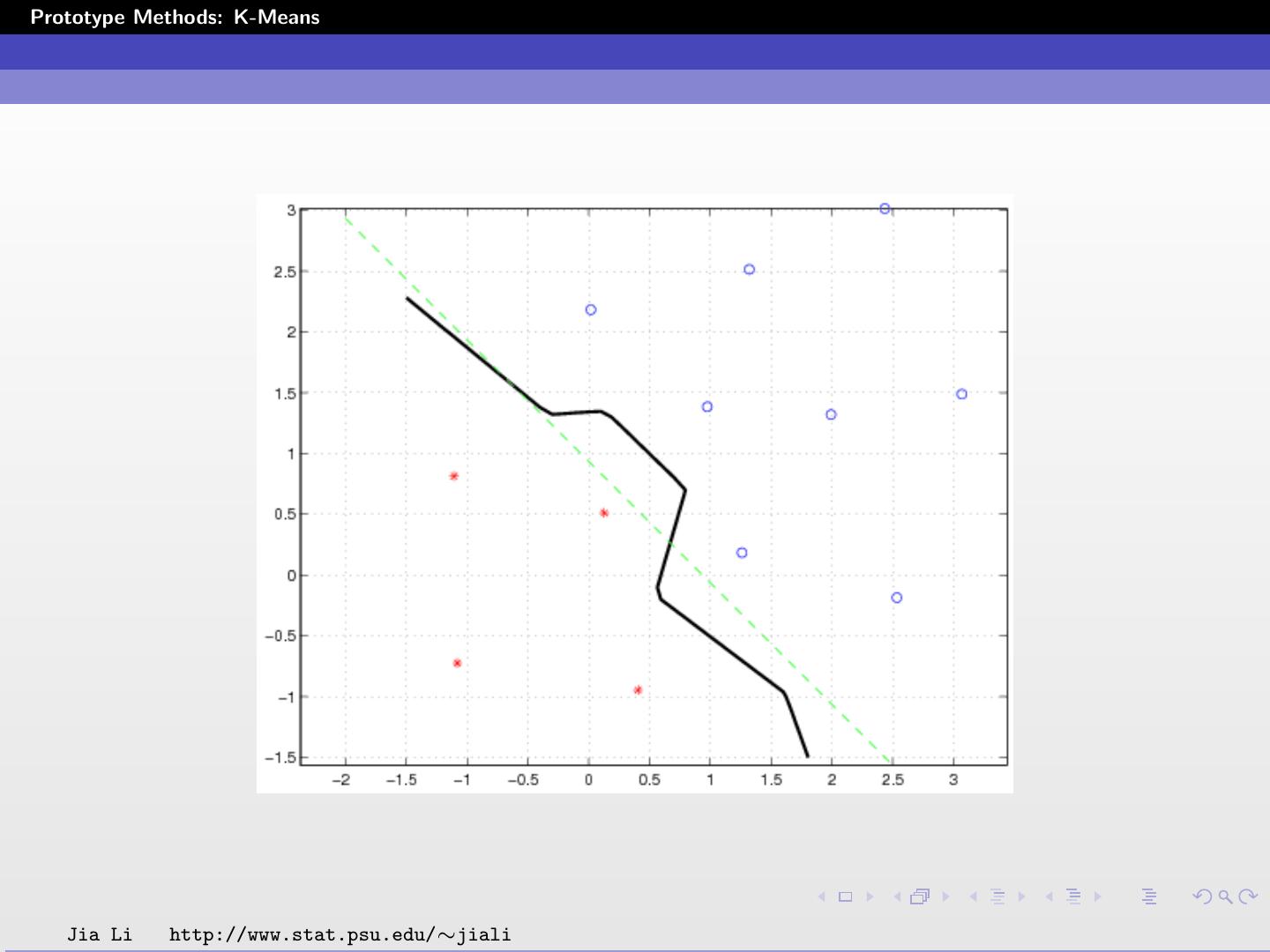
16 .Prototype Methods: K-Means K-means with Scheme 2 For the entire training data set, use M = 12 prototypes. By counting the number of samples from each class that fall into each prototype, 4 prototypes are labeled as Class 1 and the other 8 are labeled as Class 2. The prototypes for each class are shown below. The black solid line is the boundary between the two classes given by K-means. The green dash line is the optimal decision boundary. The error rate based on the test data is 13.15%. Jia Li http://www.stat.psu.edu/∼jiali 

17 .Prototype Methods: K-Means Jia Li http://www.stat.psu.edu/∼jiali 

18 .Prototype Methods: K-Means Compare the Two Schemes Scheme 1 works when there is a small amount of overlap between classes. Scheme 2 is more robust when there is a considerable amount of overlap. For Scheme 2, there is no need to specify the number of prototypes for each class separately. The number of prototypes assigned to each class is adjusted automatically. Classes with higher priors tend to occupy more prototypes. Jia Li http://www.stat.psu.edu/∼jiali 

19 .Prototype Methods: K-Means Scheme 2 has better statistical interpretation. Attempt to estimate Pr (G = j | X ) by a piece-wise constant function. Partition the feature space into cells. Assume Pr (G = j | X ) constant for X in one cell. Estimate Pr (G = j | X ) by the empirical frequencies of the classes based on all the training samples that fall into this cell. Jia Li http://www.stat.psu.edu/∼jiali 

20 .Prototype Methods: K-Means Initialization Randomly pick up the prototypes to start the k-means iteration. Different initial prototypes may lead to different local optimal solutions given by k-means. Try different sets of initial prototypes, compare the objective function at the end to choose the best solution. When randomly select initial prototypes, better make sure no prototype is out of the range of the entire data set. Jia Li http://www.stat.psu.edu/∼jiali 

21 .Prototype Methods: K-Means Initialization in the above simulation: Generated M random vectors with independent dimensions. For each dimension, the feature is uniformly distributed in [−1, 1]. Linearly transform the jth feature, Zj , j = 1, 2, ..., p in each prototype (a vector) by: Zj sj + mj , where sj is the sample standard deviation of dimension j and mj is the sample mean of dimension j, both computed using the training data. Jia Li http://www.stat.psu.edu/∼jiali 

22 .Prototype Methods: K-Means Linde-Buzo-Gray (LBG) Algorithm An algorithm developed in vector quantization for the purpose of data compression. Y. Linde, A. Buzo and R. M. Gray, ”An algorithm for vector quantizer design,” IEEE Trans. on Communication, Vol. COM-28, pp. 84-95, Jan. 1980. Jia Li http://www.stat.psu.edu/∼jiali 

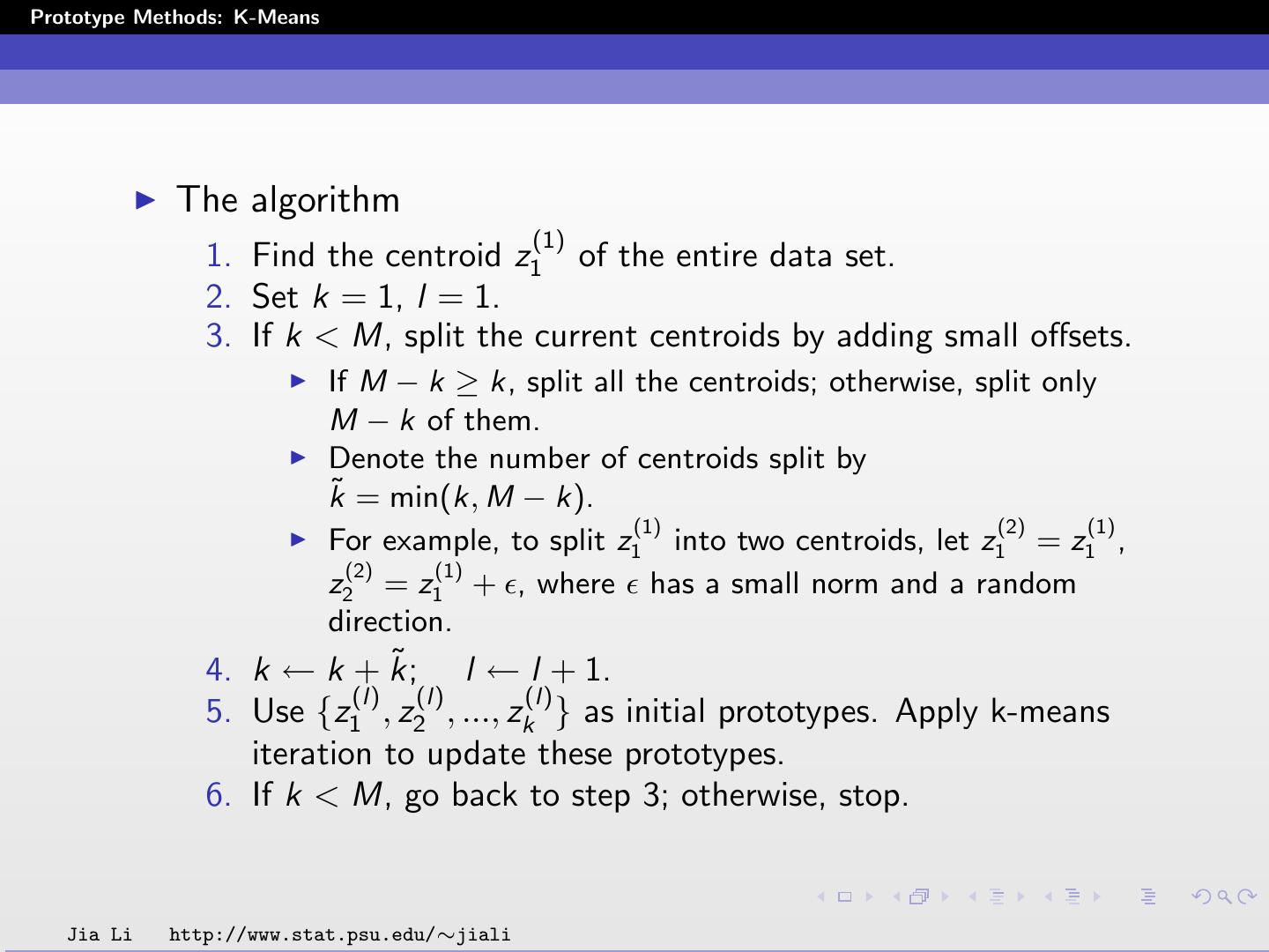
23 .Prototype Methods: K-Means The algorithm (1) 1. Find the centroid z1 of the entire data set. 2. Set k = 1, l = 1. 3. If k < M, split the current centroids by adding small offsets. If M − k ≥ k, split all the centroids; otherwise, split only M − k of them. Denote the number of centroids split by k˜ = min(k, M − k). (1) (2) (1) For example, to split z1 into two centroids, let z1 = z1 , (2) (1) z2 = z1 + , where has a small norm and a random direction. 4. k ← k + k; ˜ l ← l + 1. (l) (l) (l) 5. Use {z1 , z2 , ..., zk } as initial prototypes. Apply k-means iteration to update these prototypes. 6. If k < M, go back to step 3; otherwise, stop. Jia Li http://www.stat.psu.edu/∼jiali 

24 .Prototype Methods: K-Means Tree-structured Vector Quantization (TSVQ) for Clustering 1. Apply 2 centroids k-means to the entire data set. 2. The data are assigned to the 2 centroids. 3. For the data assigned to each centroid, apply 2 centroids k-means to them separately. 4. Repeat the above step. Jia Li http://www.stat.psu.edu/∼jiali 

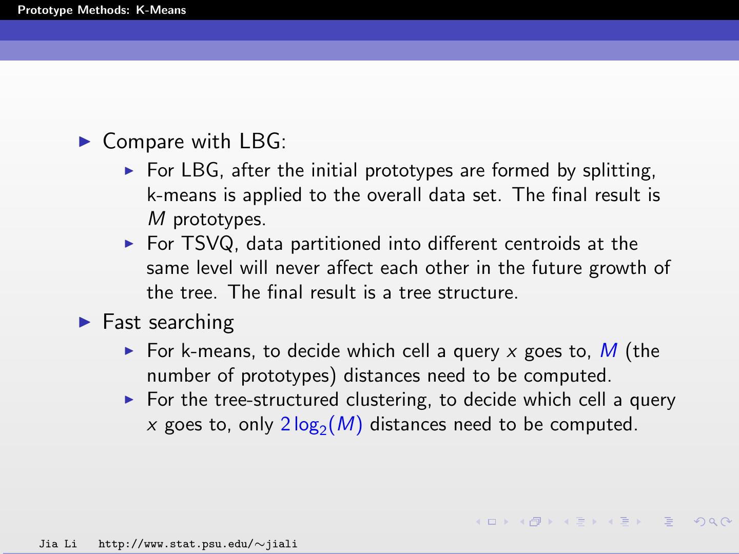
25 .Prototype Methods: K-Means Compare with LBG: For LBG, after the initial prototypes are formed by splitting, k-means is applied to the overall data set. The final result is M prototypes. For TSVQ, data partitioned into different centroids at the same level will never affect each other in the future growth of the tree. The final result is a tree structure. Fast searching For k-means, to decide which cell a query x goes to, M (the number of prototypes) distances need to be computed. For the tree-structured clustering, to decide which cell a query x goes to, only 2 log2 (M) distances need to be computed. Jia Li http://www.stat.psu.edu/∼jiali 

26 .Prototype Methods: K-Means Comments on tree-structured clustering: It is structurally more constrained. But on the other hand, it provides more insight into the patterns in the data. It is greedy in the sense of optimizing at each step sequentially. An early bad decision will propagate its effect. It provides more algorithmic flexibility. Jia Li http://www.stat.psu.edu/∼jiali 

27 .Prototype Methods: K-Means Choose the Number of Prototypes Cross-validation (data driven approach): For different number of prototypes, compute the classification error rate using cross-validation. The number of prototypes that yields the minimum error rate according to cross-validation is selected. Cross-validation is often rather effective. Rule of thumb: on average every cell contains at least 5 ∼ 10 samples. Other model selection approaches. Jia Li http://www.stat.psu.edu/∼jiali 

28 .Prototype Methods: K-Means Example Diabetes data set. The two principal components are used. For the number of prototypes M = 1, 2, ..., 20, apply k-means to classification. Two-fold cross-validation is used to compute the error rates. The error rate vs. M is plotted below. When M ≥ 8, the performance is close. The minimum error rate 27.34% is achieved by M = 13. Jia Li http://www.stat.psu.edu/∼jiali 

29 .Prototype Methods: K-Means Jia Li http://www.stat.psu.edu/∼jiali