linear methods for classification

1 .Linear Methods for Classification Linear Methods for Classification Jia Li Department of Statistics The Pennsylvania State University Email: jiali@stat.psu.edu http://www.stat.psu.edu/∼jiali Jia Li http://www.stat.psu.edu/∼jiali 

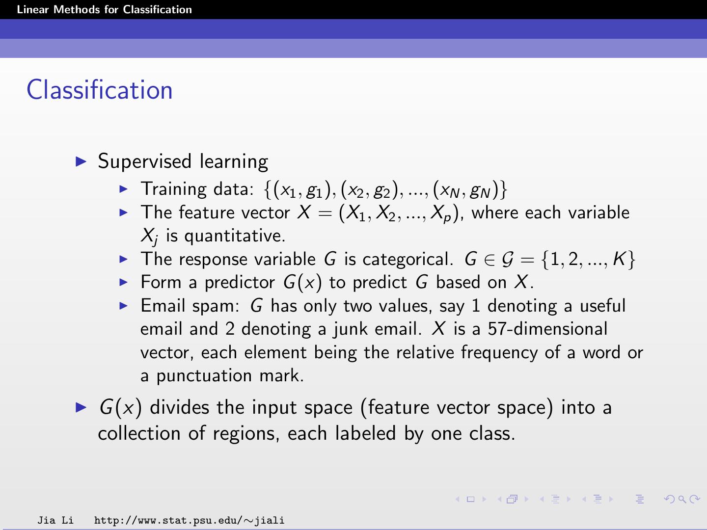
2 .Linear Methods for Classification Classification Supervised learning Training data: {(x1 , g1 ), (x2 , g2 ), ..., (xN , gN )} The feature vector X = (X1 , X2 , ..., Xp ), where each variable Xj is quantitative. The response variable G is categorical. G ∈ G = {1, 2, ..., K } Form a predictor G (x) to predict G based on X . Email spam: G has only two values, say 1 denoting a useful email and 2 denoting a junk email. X is a 57-dimensional vector, each element being the relative frequency of a word or a punctuation mark. G (x) divides the input space (feature vector space) into a collection of regions, each labeled by one class. Jia Li http://www.stat.psu.edu/∼jiali 

3 .Linear Methods for Classification Jia Li http://www.stat.psu.edu/∼jiali 

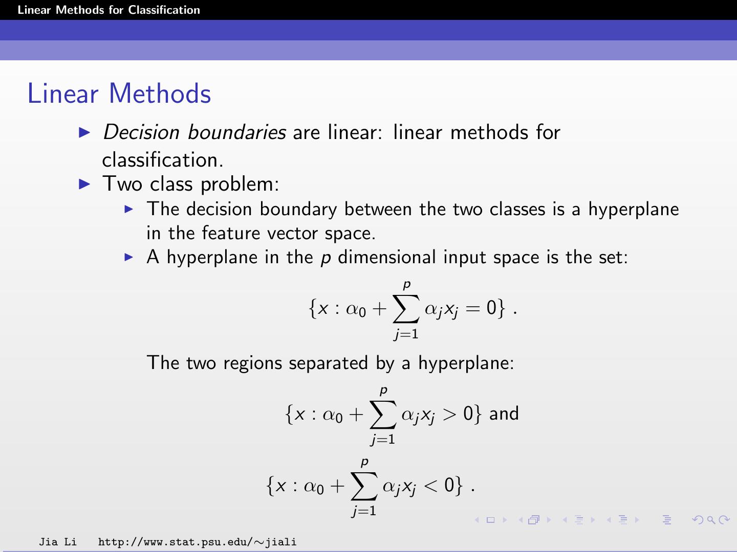
4 .Linear Methods for Classification Linear Methods Decision boundaries are linear: linear methods for classification. Two class problem: The decision boundary between the two classes is a hyperplane in the feature vector space. A hyperplane in the p dimensional input space is the set: p {x : α0 + αj xj = 0} . j=1 The two regions separated by a hyperplane: p {x : α0 + αj xj > 0} and j=1 p {x : α0 + αj xj < 0} . j=1 Jia Li http://www.stat.psu.edu/∼jiali 

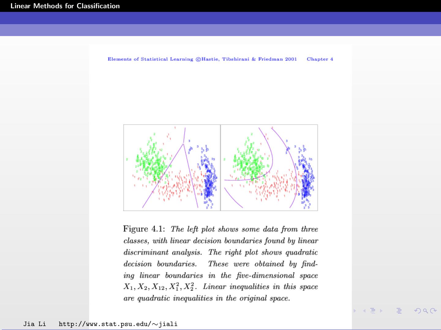
5 .Linear Methods for Classification More than two classes: The decision boundary between any pair of class k and l is a hyperplane (shown in previous figure). Question: which hyperplanes to use? Different criteria lead to different algorithms. Linear regression of an indicator matrix. Linear discriminant analysis. Logistic regression. Rosenblatt’s perceptron learning algorithm. Linear decision boundaries are not necessarily constrained. Jia Li http://www.stat.psu.edu/∼jiali 

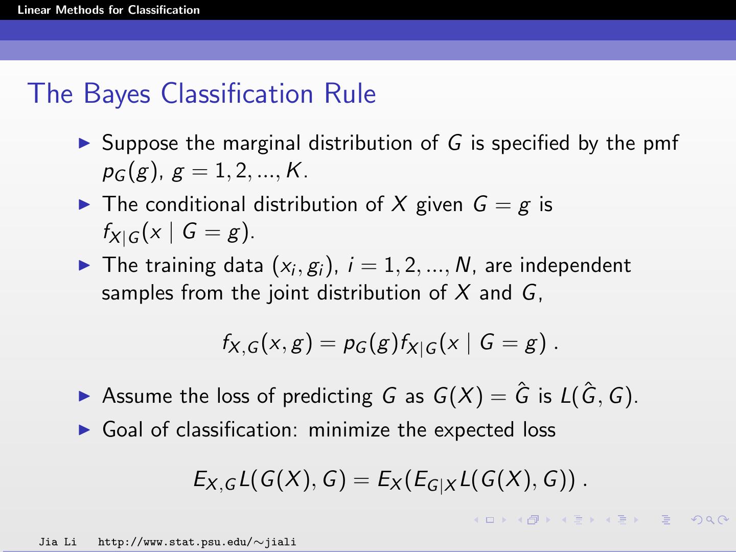
6 .Linear Methods for Classification The Bayes Classification Rule Suppose the marginal distribution of G is specified by the pmf pG (g ), g = 1, 2, ..., K . The conditional distribution of X given G = g is fX |G (x | G = g ). The training data (xi , gi ), i = 1, 2, ..., N, are independent samples from the joint distribution of X and G , fX ,G (x, g ) = pG (g )fX |G (x | G = g ) . ˆ is L(G Assume the loss of predicting G as G (X ) = G ˆ , G ). Goal of classification: minimize the expected loss EX ,G L(G (X ), G ) = EX (EG |X L(G (X ), G )) . Jia Li http://www.stat.psu.edu/∼jiali 

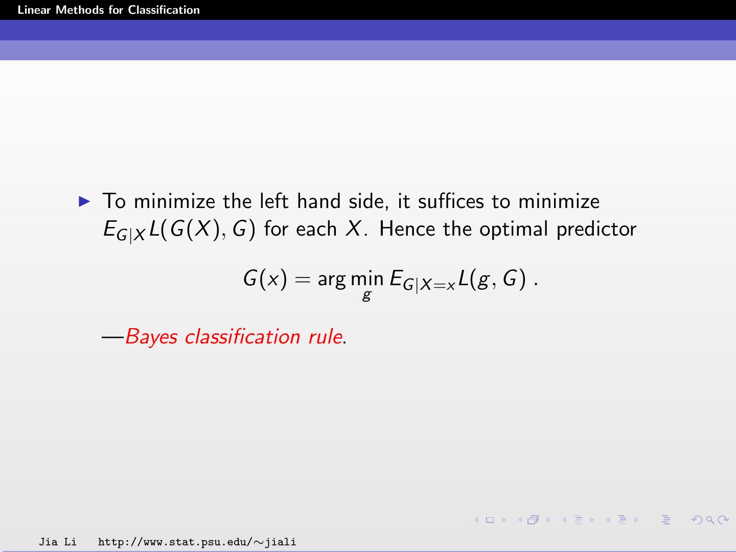
7 .Linear Methods for Classification To minimize the left hand side, it suffices to minimize EG |X L(G (X ), G ) for each X . Hence the optimal predictor G (x) = arg min EG |X =x L(g , G ) . g —Bayes classification rule. Jia Li http://www.stat.psu.edu/∼jiali 

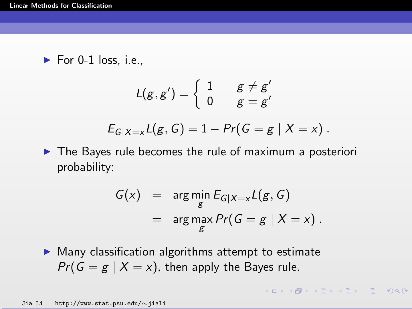
8 .Linear Methods for Classification For 0-1 loss, i.e., 1 g =g L(g , g ) = 0 g =g EG |X =x L(g , G ) = 1 − Pr (G = g | X = x) . The Bayes rule becomes the rule of maximum a posteriori probability: G (x) = arg min EG |X =x L(g , G ) g = arg max Pr (G = g | X = x) . g Many classification algorithms attempt to estimate Pr (G = g | X = x), then apply the Bayes rule. Jia Li http://www.stat.psu.edu/∼jiali 

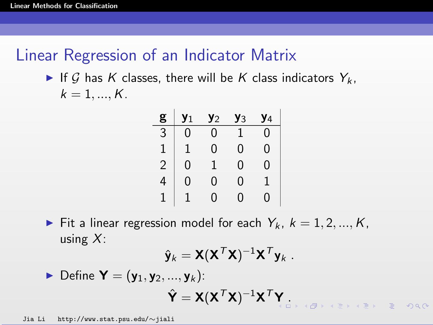
9 .Linear Methods for Classification Linear Regression of an Indicator Matrix If G has K classes, there will be K class indicators Yk , k = 1, ..., K . g y1 y2 y3 y4 3 0 0 1 0 1 1 0 0 0 2 0 1 0 0 4 0 0 0 1 1 1 0 0 0 Fit a linear regression model for each Yk , k = 1, 2, ..., K , using X : yˆk = X(XT X)−1 XT yk . Define Y = (y1 , y2 , ..., yk ): Yˆ = X(XT X)−1 XT Y . Jia Li http://www.stat.psu.edu/∼jiali 

10 .Linear Methods for Classification Classification Procedure ˆ = (XT X)−1 XT Y. Define B For a new observation with input x, compute the fitted output fˆ(x) = [(1, x)B] ˆ T ˆ T = [(1, x1 , x2 , ..., xp )B]  ˆ  f1 (x)  fˆ2 (x)  =   ...   fˆK (x) Identify the largest component of fˆ(x) and classify accordingly: Gˆ (x) = arg max fˆk (x) . k∈G Jia Li http://www.stat.psu.edu/∼jiali 

11 .Linear Methods for Classification Rationale The linear regression of Yk on X is a linear approximation to E (Yk | X = x). E (Yk | X = x) = Pr (Yk = 1 | X = x) · 1 + Pr (Yk = 0 | X = x) · 0 = Pr (Yk = 1 | X = x) = Pr (G = k | X = x) According to the Bayes rule, the optimal classifier: G ∗ (x) = arg max Pr (G = k | X = x) . k∈G Linear regression of an indicator matrix: Approximate Pr (G = k | X = x) by a linear function of x using linear regression. Apply the Bayes rule to the approximated probability. Jia Li http://www.stat.psu.edu/∼jiali 

12 .Linear Methods for Classification Example: Diabetes Data The diabetes data set is taken from the UCI machine learning database repository at: http://www.ics.uci.edu/˜mlearn/Machine-Learning.html . The original source of the data is the National Institute of Diabetes and Digestive and Kidney Diseases. There are 768 cases in the data set, of which 268 show signs of diabetes according to World Health Organization criteria. Each case contains 8 quantitative variables, including diastolic blood pressure, triceps skin fold thickness, a body mass index, etc. Two classes: with or without signs of diabetes. ˜1 , X Denote the 8 original variables by X ˜2 , ..., X ˜8 . ˜j and normalize it to unit variance. Remove the mean of X Jia Li http://www.stat.psu.edu/∼jiali 

13 .Linear Methods for Classification The two principal components X1 and X2 are used in classification: ˜1 + 0.3931X X1 = 0.1284X ˜2 + 0.3600X˜3 + 0.4398X˜4 +0.4350X˜5 + 0.4519X˜6 + 0.2706X˜7 + 0.1980X˜8 ˜1 + 0.1740X X2 = 0.5938X ˜2 + 0.1839X˜3 − 0.3320X˜4 −0.2508X˜5 − 0.1010X˜6 − 0.1221X˜7 + 0.6206X˜8 Jia Li http://www.stat.psu.edu/∼jiali 

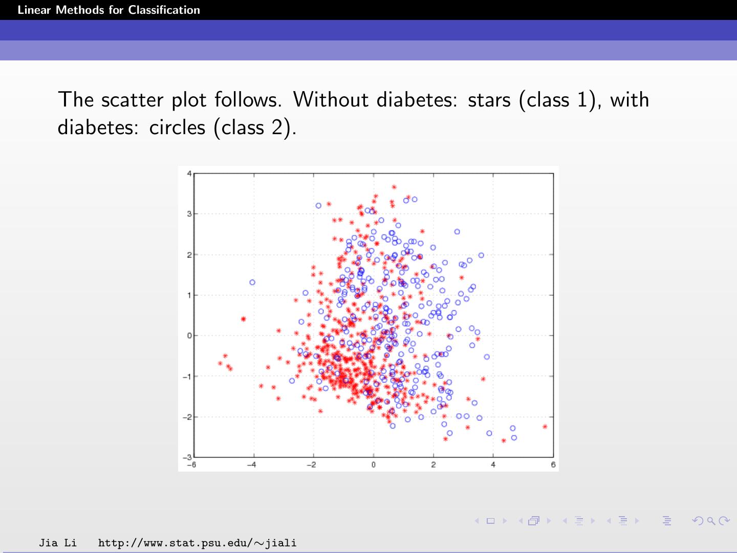
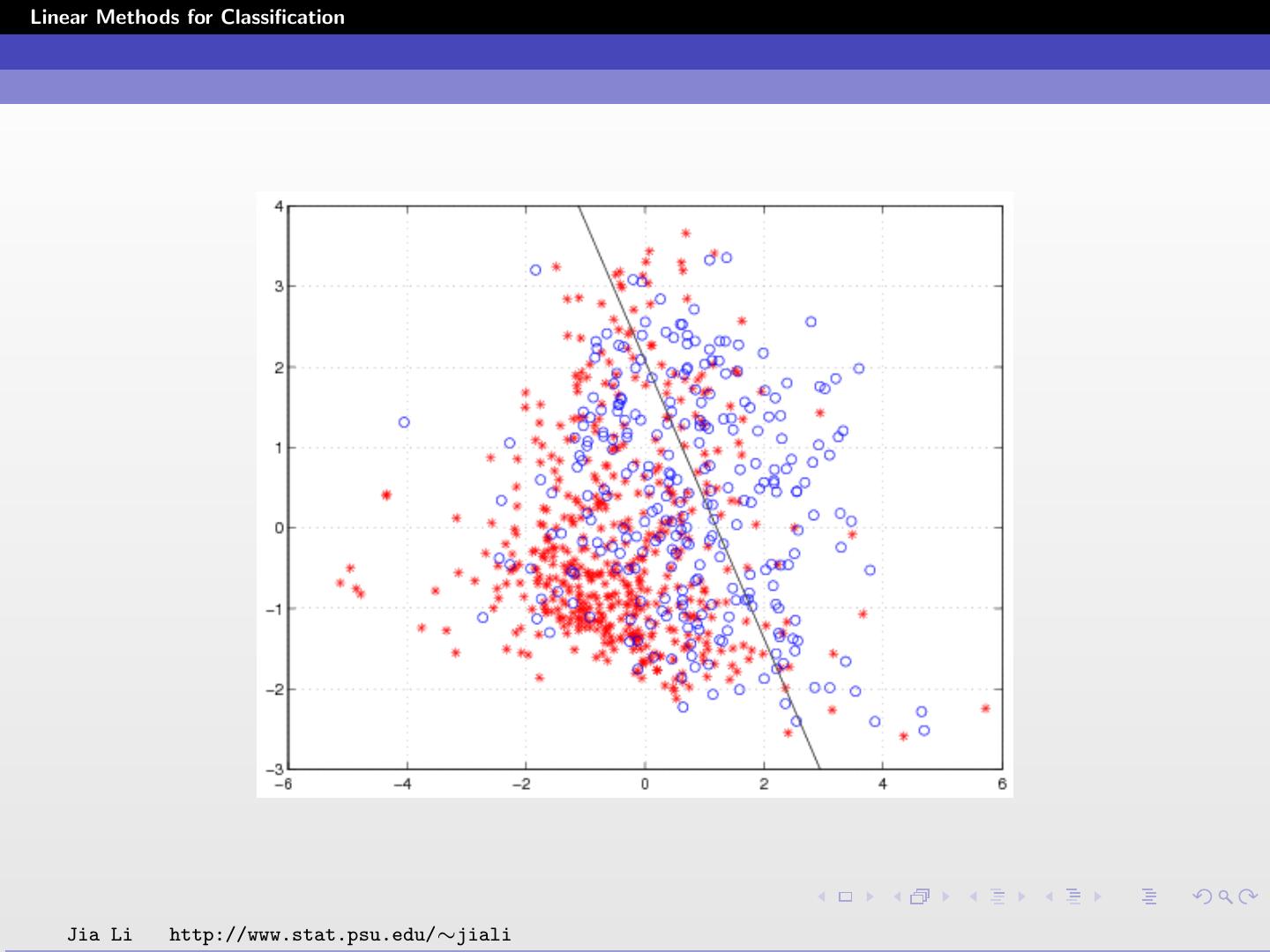
14 .Linear Methods for Classification The scatter plot follows. Without diabetes: stars (class 1), with diabetes: circles (class 2). Jia Li http://www.stat.psu.edu/∼jiali 

15 .Linear Methods for Classification ˆ = (XT X)−1 XT Y B   0.6510 0.3490 =  −0.1256 0.1256  −0.0729 0.0729 Yˆ1 = 0.6510 − 0.1256X1 − 0.0729X2 Yˆ2 = 0.3490 + 0.1256X1 + 0.0729X2 Note Yˆ1 + Yˆ2 = 1. Jia Li http://www.stat.psu.edu/∼jiali 

16 .Linear Methods for Classification Classification rule ˆ (x) = 1 Yˆ1 ≥ Yˆ2 G 2 Yˆ1 < Yˆ2 1 0.151 − 0.1256X1 − 0.0729X2 ≥ 0 = 2 otherwise Within training data classification error rate: 28.52%. Sensitivity (probability of claiming positive when the truth is positive): 44.03%. Specificity (probability of claiming negative when the truth is negative): 86.20%. Jia Li http://www.stat.psu.edu/∼jiali 

17 .Linear Methods for Classification Jia Li http://www.stat.psu.edu/∼jiali 

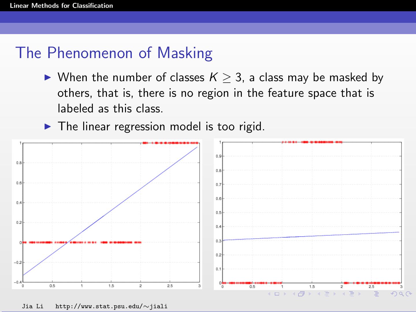
18 .Linear Methods for Classification The Phenomenon of Masking When the number of classes K ≥ 3, a class may be masked by others, that is, there is no region in the feature space that is labeled as this class. The linear regression model is too rigid. Jia Li http://www.stat.psu.edu/∼jiali 

19 .Linear Methods for Classification Jia Li http://www.stat.psu.edu/∼jiali 

20 .Linear Methods for Classification Jia Li http://www.stat.psu.edu/∼jiali