- 快召唤伙伴们来围观吧
- 微博 QQ QQ空间 贴吧
- 文档嵌入链接
- 复制
- 微信扫一扫分享
- 已成功复制到剪贴板
classification_performance_measures.pptx
展开查看详情
1 .Evaluating Classification Performance Data Mining 1
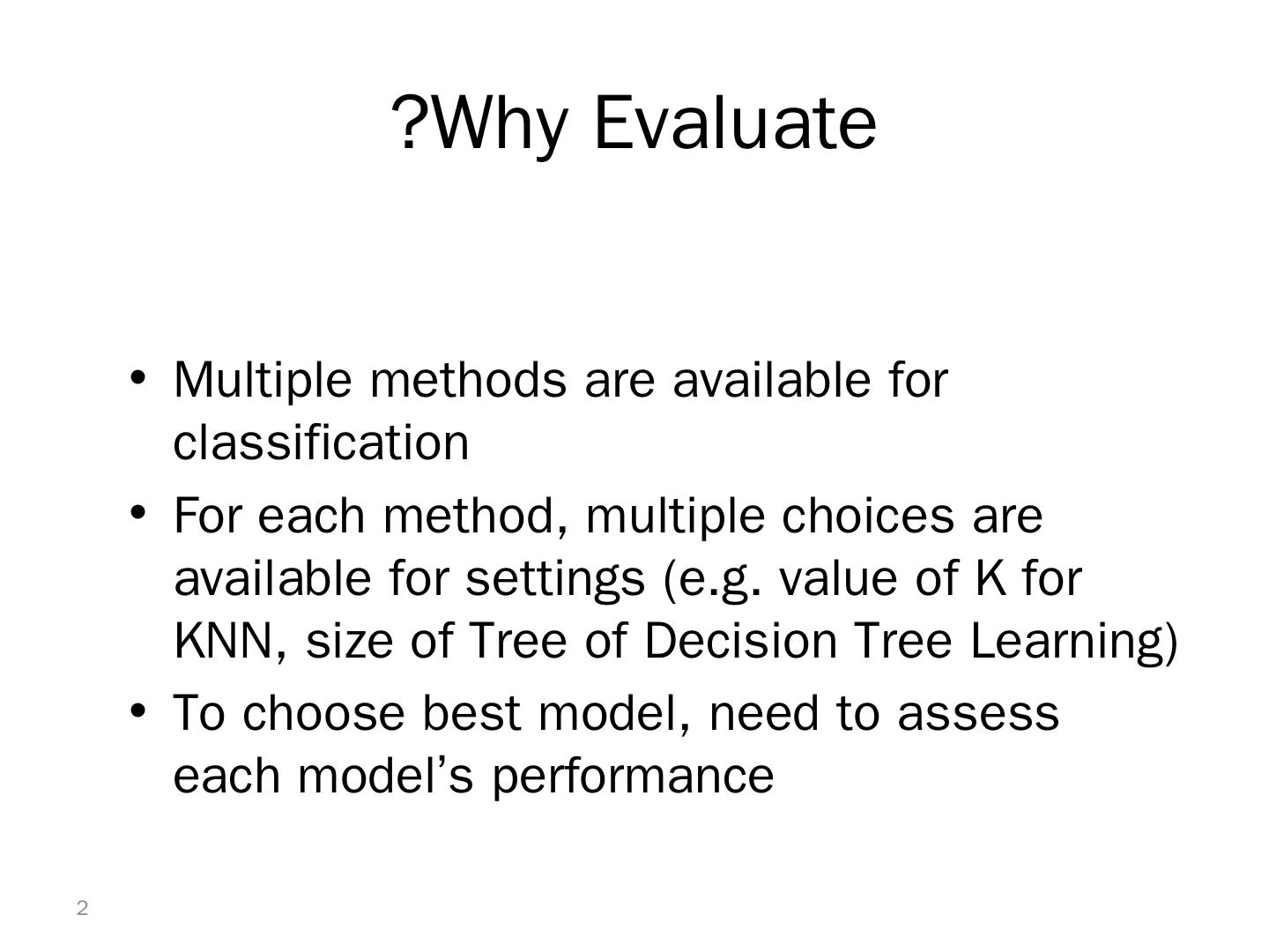
2 .Why Evaluate? Multiple methods are available for classification For each method, multiple choices are available for settings (e.g. value of K for KNN, size of Tree of Decision Tree Learning) To choose best model, need to assess each model’s performance 2
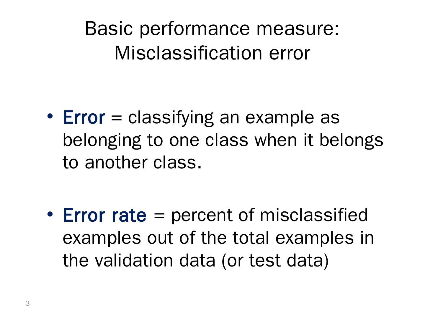
3 .Basic performance measure: Misclassification error Error = classifying an example as belonging to one class when it belongs to another class. Error rate = percent of misclassified examples out of the total examples in the validation data (or test data) 3
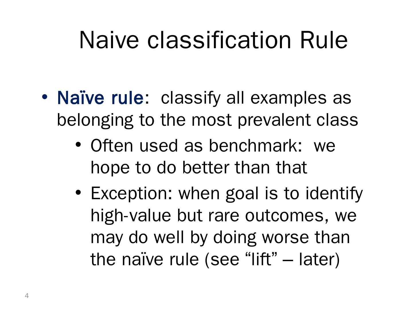
4 .Naive classification Rule Naïve rule : classify all examples as belonging to the most prevalent class Often used as benchmark: we hope to do better than that Exception: when goal is to identify high-value but rare outcomes, we may do well by doing worse than the naïve rule (see “lift” – later) 4
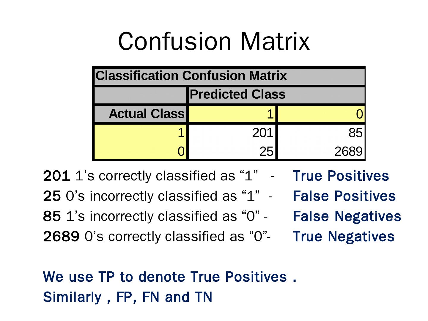
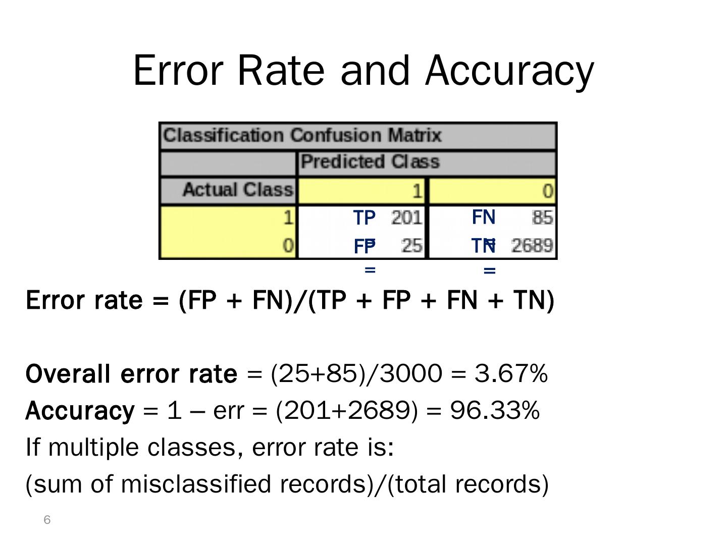
5 .Confusion Matrix 201 1’s correctly classified as “1” - True Positives 25 0’s incorrectly classified as “1 ” - False Positives 85 1’s incorrectly classified as “0” - False Negatives 2689 0’s correctly classified as “0”- True Negatives We use TP to denote True Positives . Similarly , FP, FN and TN
6 .Error Rate and Accuracy Error rate = (FP + FN)/(TP + FP + FN + TN) Overall error rate = (25+85)/3000 = 3.67% Accuracy = 1 – err = (201+2689) = 96.33% If multiple classes, error rate is: (sum of misclassified records)/(total records) 6 TP = FN = FP = TN =
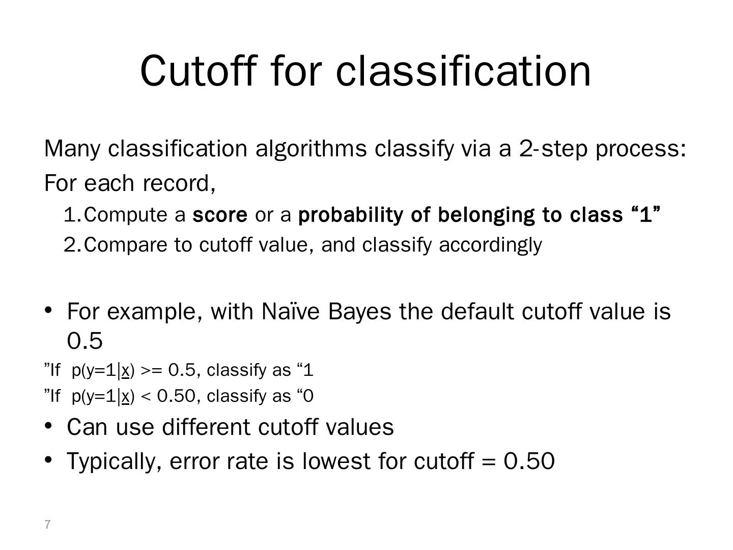
7 .Cutoff for classification Many classification algorithms classify via a 2-step process: For each record, Compute a score or a probability of belonging to class “1” Compare to cutoff value, and classify accordingly For example, with Naïve Bayes the default cutoff value is 0.5 If p(y=1| x ) >= 0.5, classify as “1” If p(y=1| x ) < 0.50, classify as “0” Can use different cutoff values Typically, error rate is lowest for cutoff = 0.50 7
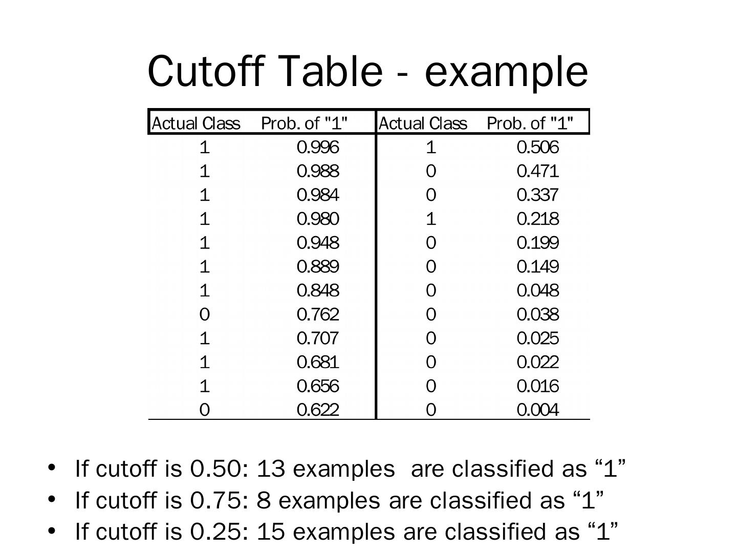
8 .Cutoff Table - example If cutoff is 0.50: 13 examples are classified as “1” If cutoff is 0.75: 8 example s are classified as “1” If cutoff is 0.25 : 15 examples are classified as “1”
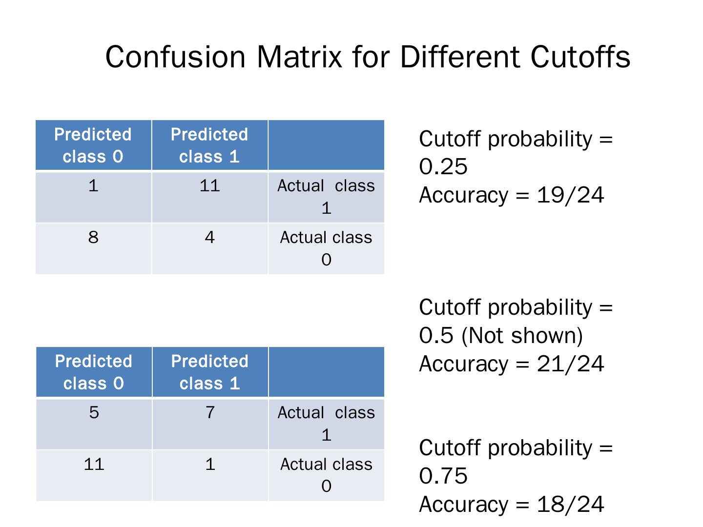
9 .Confusion Matrix for Different Cutoffs Predicted class 0 Predicted class 1 1 11 Actual class 1 8 4 Actual class 0 Cutoff probability = 0.25 Accuracy = 19/24 Cutoff probability = 0.5 (Not shown) Accuracy = 21/24 Cutoff probability = 0.75 Accuracy = 18/24 Predicted class 0 Predicted class 1 5 7 Actual class 1 11 1 Actual class 0
10 .Lift 10
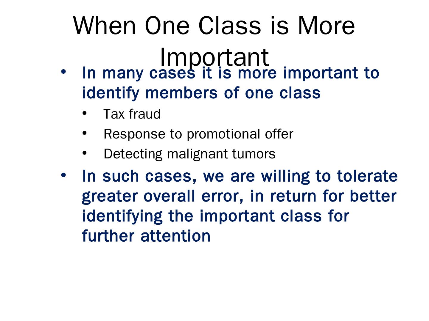
11 .When One Class is More Important In many cases it is more important to identify members of one class Tax fraud Response to promotional offer Detecting malignant tumors In such cases, we are willing to tolerate greater overall error, in return for better identifying the important class for further attention
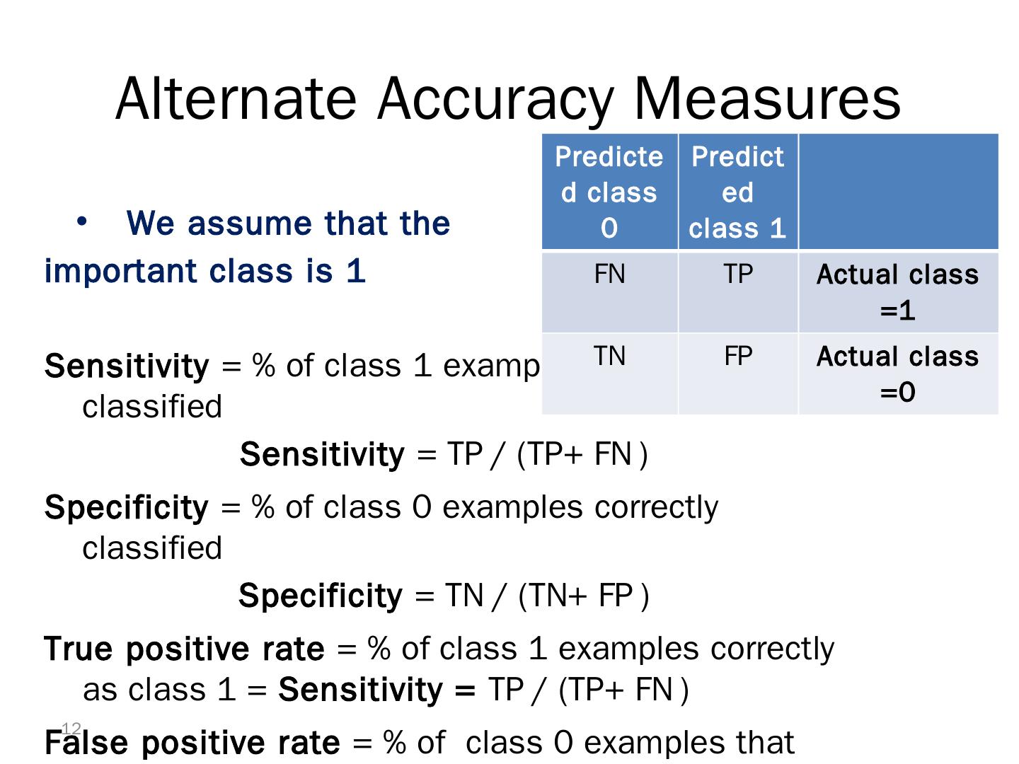
12 .Alternate Accuracy Measures We assume that the important class is 1 Sensitivity = % of class 1 examples correctly classified Sensitivity = TP / (TP+ FN ) Specificity = % of class 0 examples correctly classified Specificity = TN / (TN+ FP ) True positive rate = % of class 1 examples correctly as class 1 = Sensitivity = TP / (TP+ FN ) False positive rate = % of class 0 examples that were classified as class 1 = 1- specificity = FP / (TN+ FP ) 12 Predicted class 0 Predicted class 1 FN TP Actual class =1 TN FP Actual class =0
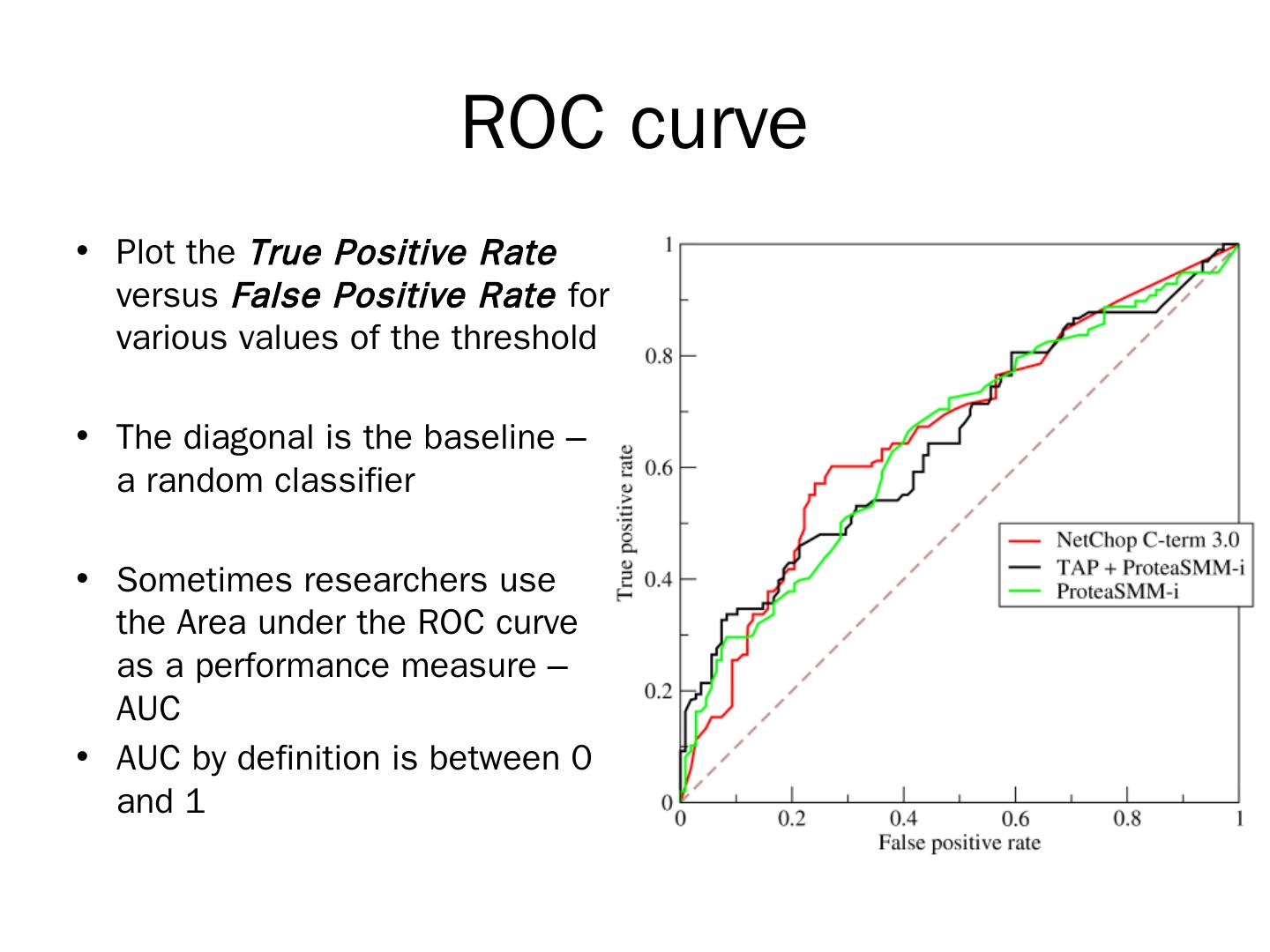
13 .ROC curve Plot the True Positive Rate versus False Positive Rate for various values of the threshold The diagonal is the baseline – a random classifier Sometimes researchers use the Area under the ROC curve as a performance measure – AUC AUC by definition is between 0 and 1
14 .Lift Charts: Goal Useful for assessing performance in terms of identifying the most important class Helps evaluate, e.g., How many tax records to examine How many loans to grant How many customers to mail offer to 14
15 .Lift Charts – Cont. Compare performance of DM model to “no model, pick randomly” Measures ability of DM model to identify the important class, relative to its average prevalence Charts give explicit assessment of results over a large number of cutoffs 15
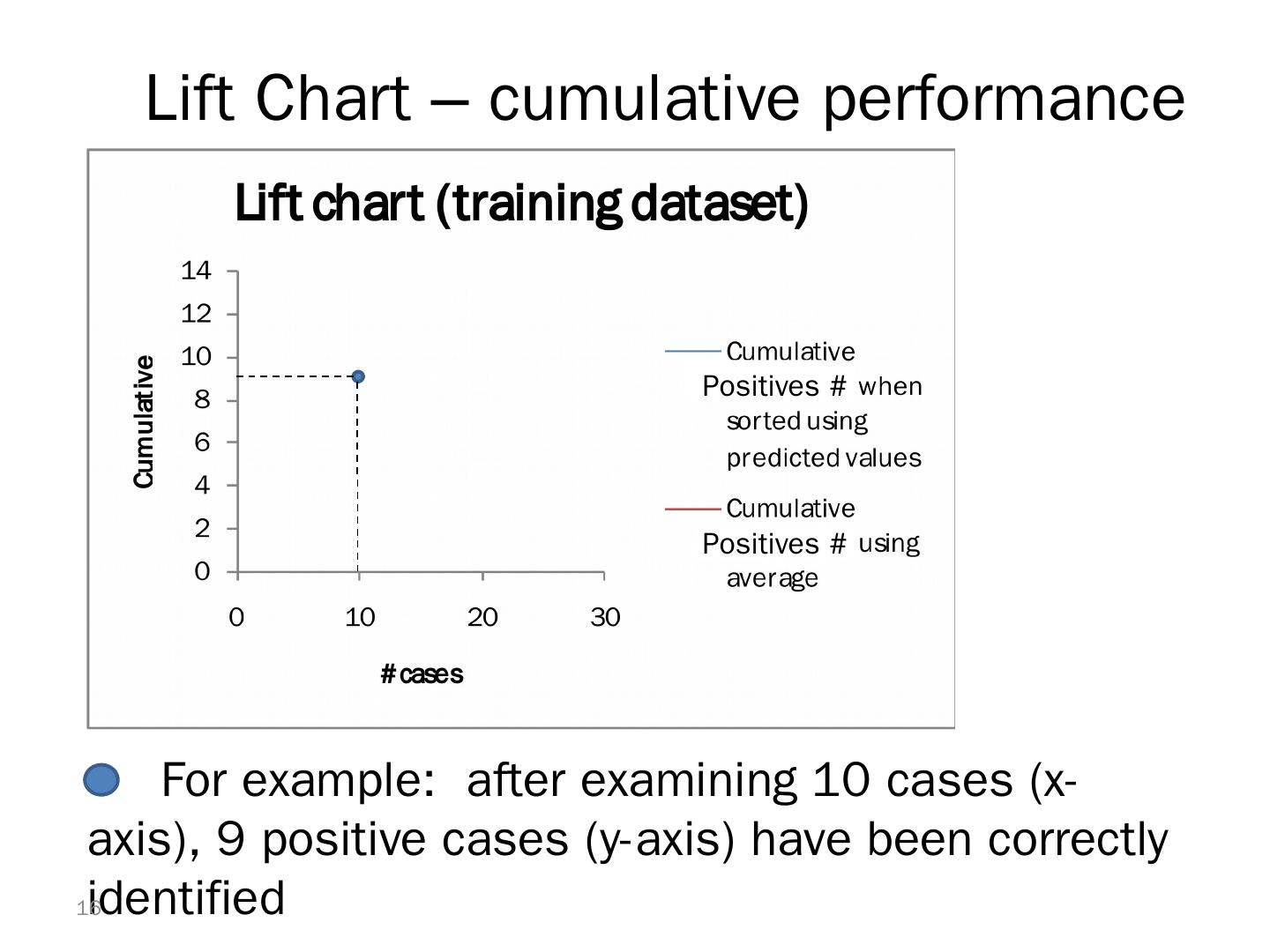
16 .Lift Chart – cumulative performance For example: after examining 10 cases (x-axis), 9 positive cases (y-axis) have been correctly identified 16 Positives #Positives #Positives
17 .Lift Charts: How to Compute Using the model’s classification scores, sort examples from most likely to least likely members of the important class Compute lift: Accumulate the correctly classified “important class” records (Y axis) and compare to number of total records (X axis) 17
18 .Asymmetric Costs 18
19 .Misclassification Costs May Differ The cost of making a misclassification error may be higher for one class than the other(s) Looked at another way, the benefit of making a correct classification may be higher for one class than the other(s) 19
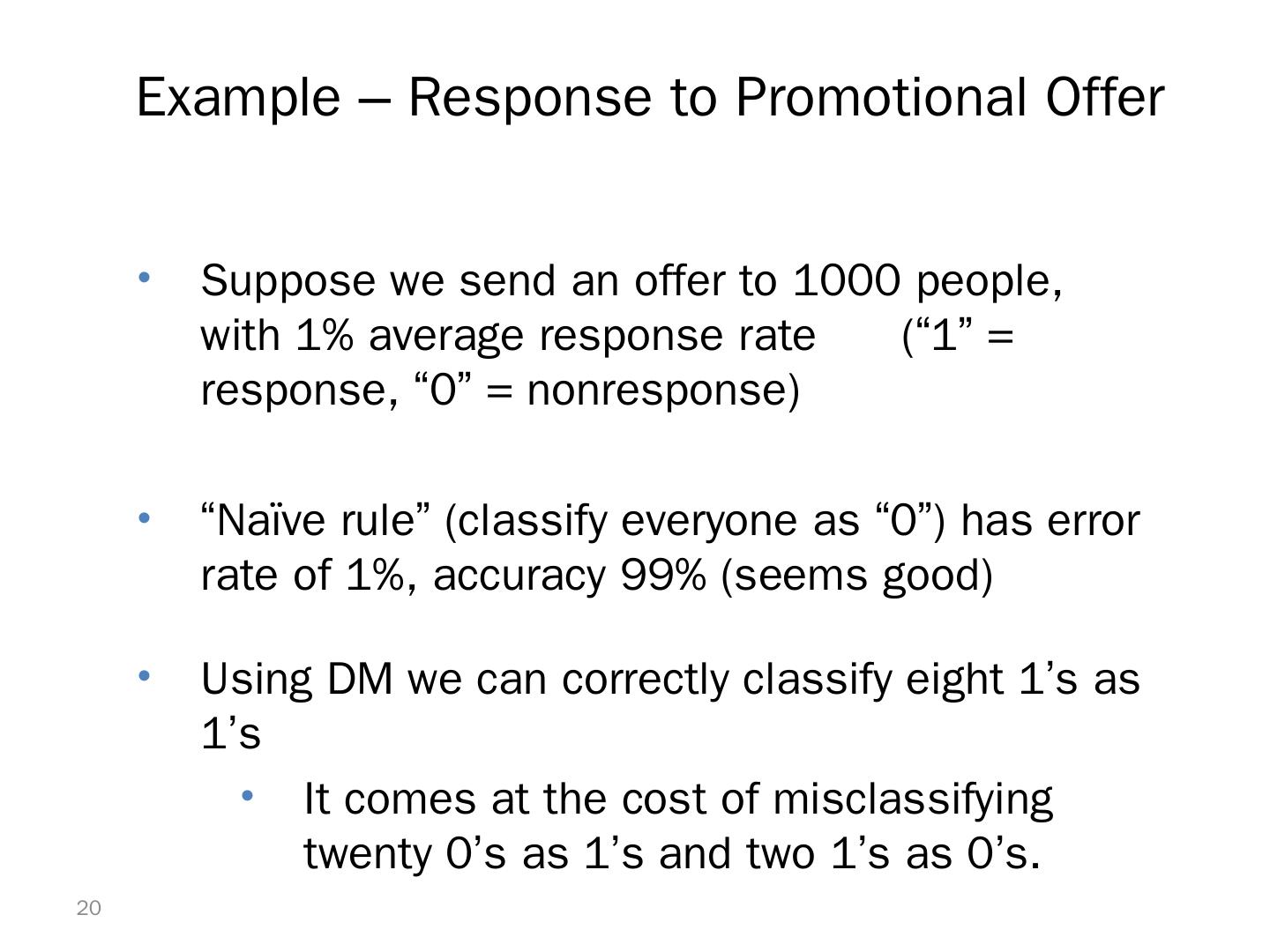
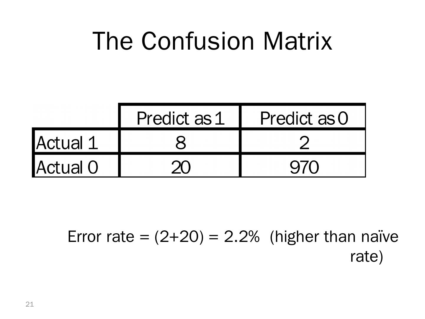
20 .Example – Response to Promotional Offer Suppose we send an offer to 1000 people, with 1% average response rate (“ 1” = response, “0” = nonresponse) “Naïve rule” (classify everyone as “0”) has error rate of 1 %, accuracy 99% (seems good) Using DM we can correctly classify eight 1’s as 1’s It comes at the cost of misclassifying twenty 0’s as 1’s and two 1’s as 0 ’s . 20
21 .The Confusion Matrix Error rate = (2+20) = 2.2% (higher than naïve rate) 21
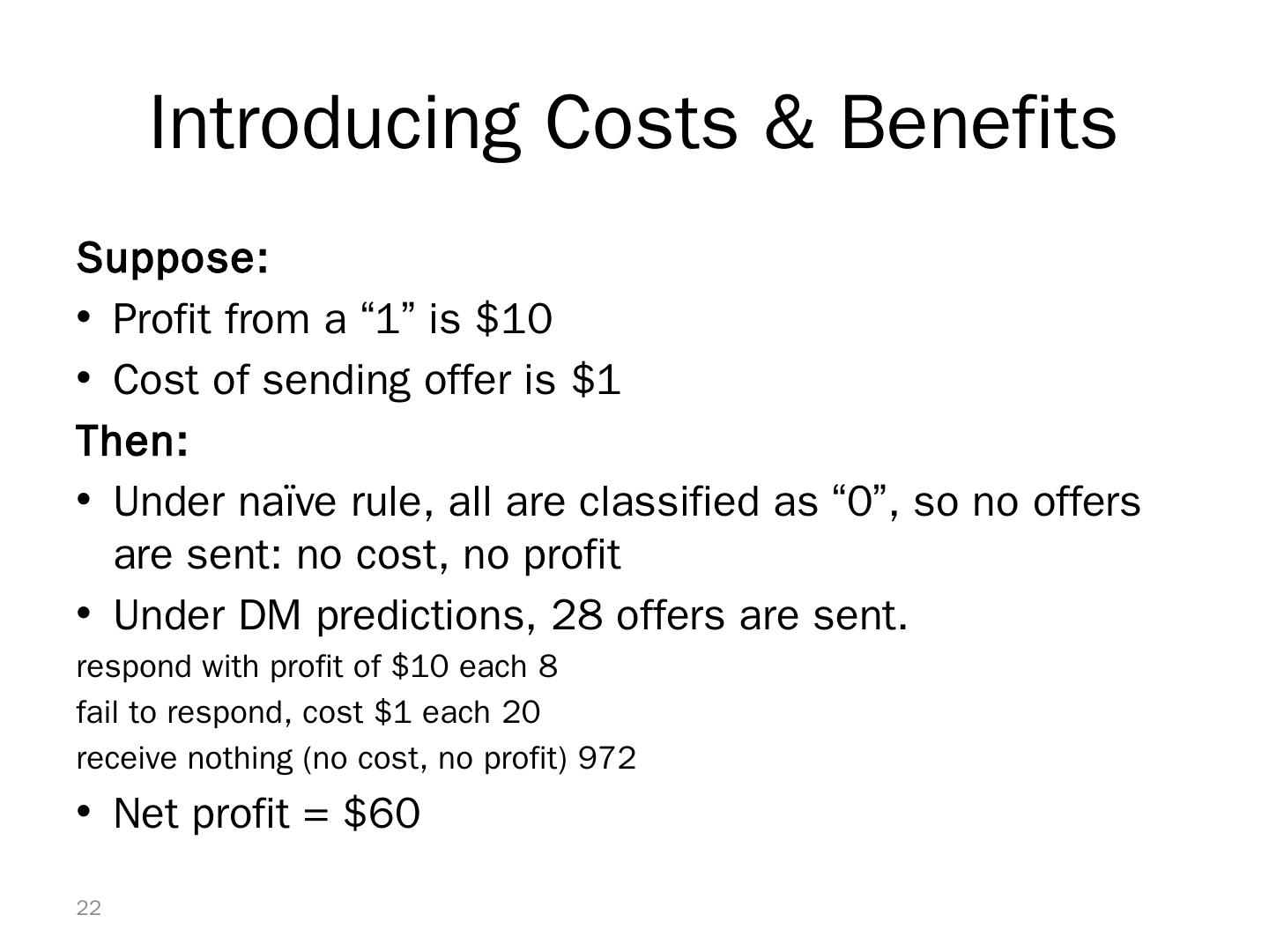
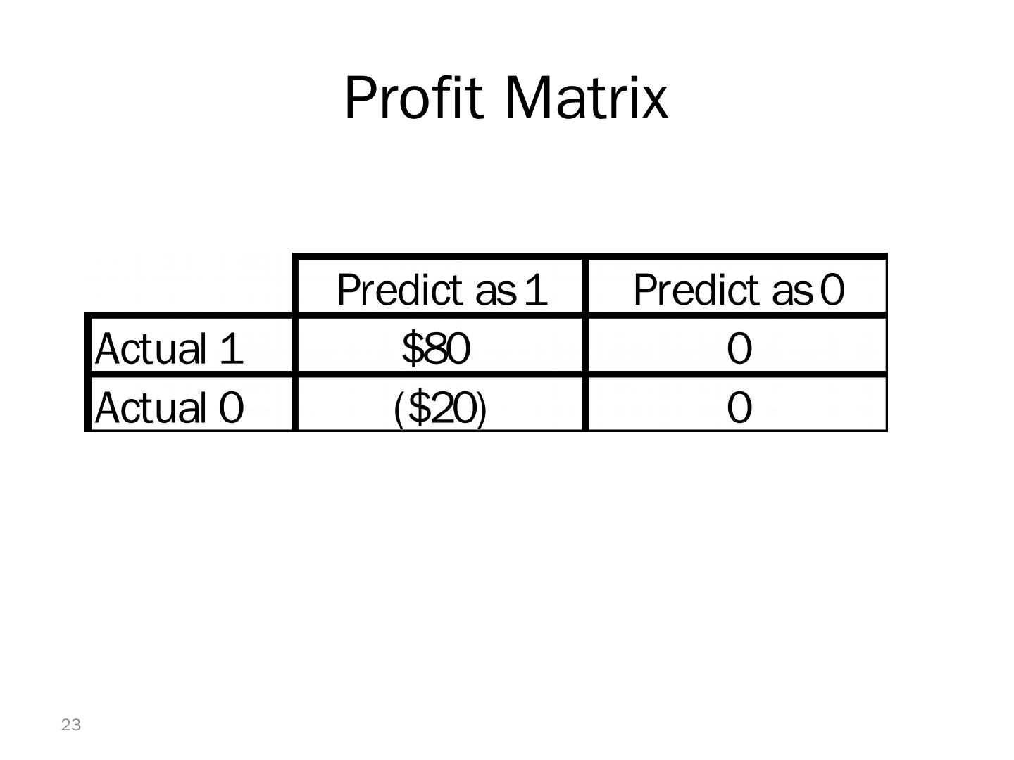
22 .Introducing Costs & Benefits Suppose: Profit from a “1” is $10 Cost of sending offer is $1 Then: Under naïve rule, all are classified as “0”, so no offers are sent: no cost, no profit Under DM predictions, 28 offers are sent. 8 respond with profit of $10 each 20 fail to respond, cost $1 each 972 receive nothing (no cost, no profit) Net profit = $60 22
23 .Profit Matrix 23
24 .Lift (again) Adding costs to the mix, as above, does not change the actual classifications. But it allows us to get a better decision (threshold) Use the lift curve and change the cutoff value for “1” to maximize profit 24
25 .Adding Cost/Benefit to Lift Curve Sort test examples in descending probability of success For each case, record cost/benefit of actual outcome Also record cumulative cost/benefit Plot all records X-axis is index number (1 for 1 st case, n for n th case) Y-axis is cumulative cost/benefit Reference line from origin to y n ( y n = total net benefit) 25
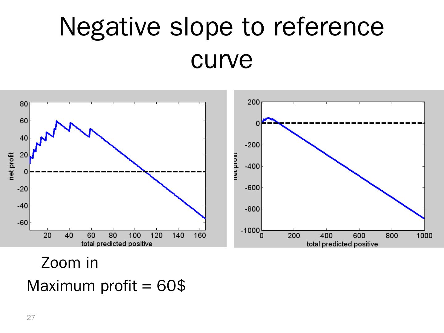
26 .Lift Curve May Go Negative If total net benefit from all cases is negative, reference line will have negative slope Nonetheless, goal is still to use cutoff to select the point where net benefit is at a maximum 26
27 .Negative slope to reference curve 27 Zoom in Maximum profit = 60$
28 .Multiple Classes Theoretically, there are m ( m -1) misclassification costs, since any case could be misclassified in m -1 ways Practically too many to work with In decision-making context, though, such complexity rarely arises – one class is usually of primary interest For m classes, confusion matrix has m rows and m columns 28
29 .Classification Using Triage Instead of classifying as C 1 or C 0 , we classify as C 1 C 0 Can’t say The third category might receive special human review Take into account a gray area in making classification decisions 29


