大数据总结

1 . What Goes Around Comes Around Michael Stonebraker Joseph M. Hellerstein Abstract This paper provides a summary of 35 years of data model proposals, grouped into 9 different eras. We discuss the proposals of each era, and show that there are only a few basic data modeling ideas, and most have been around a long time. Later proposals inevitably bear a strong resemblance to certain earlier proposals. Hence, it is a worthwhile exercise to study previous proposals. In addition, we present the lessons learned from the exploration of the proposals in each era. Most current researchers were not around for many of the previous eras, and have limited (if any) understanding of what was previously learned. There is an old adage that he who does not understand history is condemned to repeat it. By presenting “ancient history”, we hope to allow future researchers to avoid replaying history. Unfortunately, the main proposal in the current XML era bears a striking resemblance to the CODASYL proposal from the early 1970’s, which failed because of its complexity. Hence, the current era is replaying history, and “what goes around comes around”. Hopefully the next era will be smarter. I Introduction Data model proposals have been around since the late 1960’s, when the first author “came on the scene”. Proposals have continued with surprising regularity for the intervening 35 years. Moreover, many of the current day proposals have come from researchers too young to have learned from the discussion of earlier ones. Hence, the purpose of this paper is to summarize 35 years worth of “progress” and point out what should be learned from this lengthy exercise. We present data model proposals in nine historical epochs: Hierarchical (IMS): late 1960’s and 1970’s Network (CODASYL): 1970’s Relational: 1970’s and early 1980’s Entity-Relationship: 1970’s Extended Relational: 1980’s Semantic: late 1970’s and 1980’s Object-oriented: late 1980’s and early 1990’s Object-relational: late 1980’s and early 1990’s 

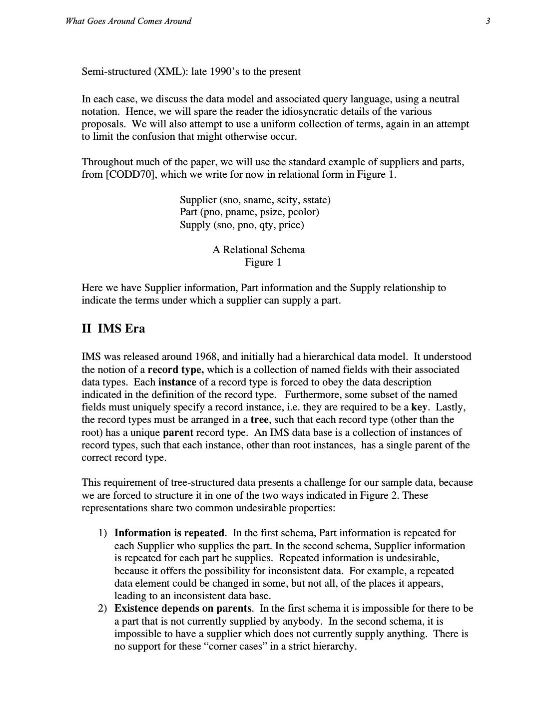
2 .What Goes Around Comes Around 3 Semi-structured (XML): late 1990’s to the present In each case, we discuss the data model and associated query language, using a neutral notation. Hence, we will spare the reader the idiosyncratic details of the various proposals. We will also attempt to use a uniform collection of terms, again in an attempt to limit the confusion that might otherwise occur. Throughout much of the paper, we will use the standard example of suppliers and parts, from [CODD70], which we write for now in relational form in Figure 1. Supplier (sno, sname, scity, sstate) Part (pno, pname, psize, pcolor) Supply (sno, pno, qty, price) A Relational Schema Figure 1 Here we have Supplier information, Part information and the Supply relationship to indicate the terms under which a supplier can supply a part. II IMS Era IMS was released around 1968, and initially had a hierarchical data model. It understood the notion of a record type, which is a collection of named fields with their associated data types. Each instance of a record type is forced to obey the data description indicated in the definition of the record type. Furthermore, some subset of the named fields must uniquely specify a record instance, i.e. they are required to be a key. Lastly, the record types must be arranged in a tree, such that each record type (other than the root) has a unique parent record type. An IMS data base is a collection of instances of record types, such that each instance, other than root instances, has a single parent of the correct record type. This requirement of tree-structured data presents a challenge for our sample data, because we are forced to structure it in one of the two ways indicated in Figure 2. These representations share two common undesirable properties: 1) Information is repeated. In the first schema, Part information is repeated for each Supplier who supplies the part. In the second schema, Supplier information is repeated for each part he supplies. Repeated information is undesirable, because it offers the possibility for inconsistent data. For example, a repeated data element could be changed in some, but not all, of the places it appears, leading to an inconsistent data base. 2) Existence depends on parents. In the first schema it is impossible for there to be a part that is not currently supplied by anybody. In the second schema, it is impossible to have a supplier which does not currently supply anything. There is no support for these “corner cases” in a strict hierarchy. 

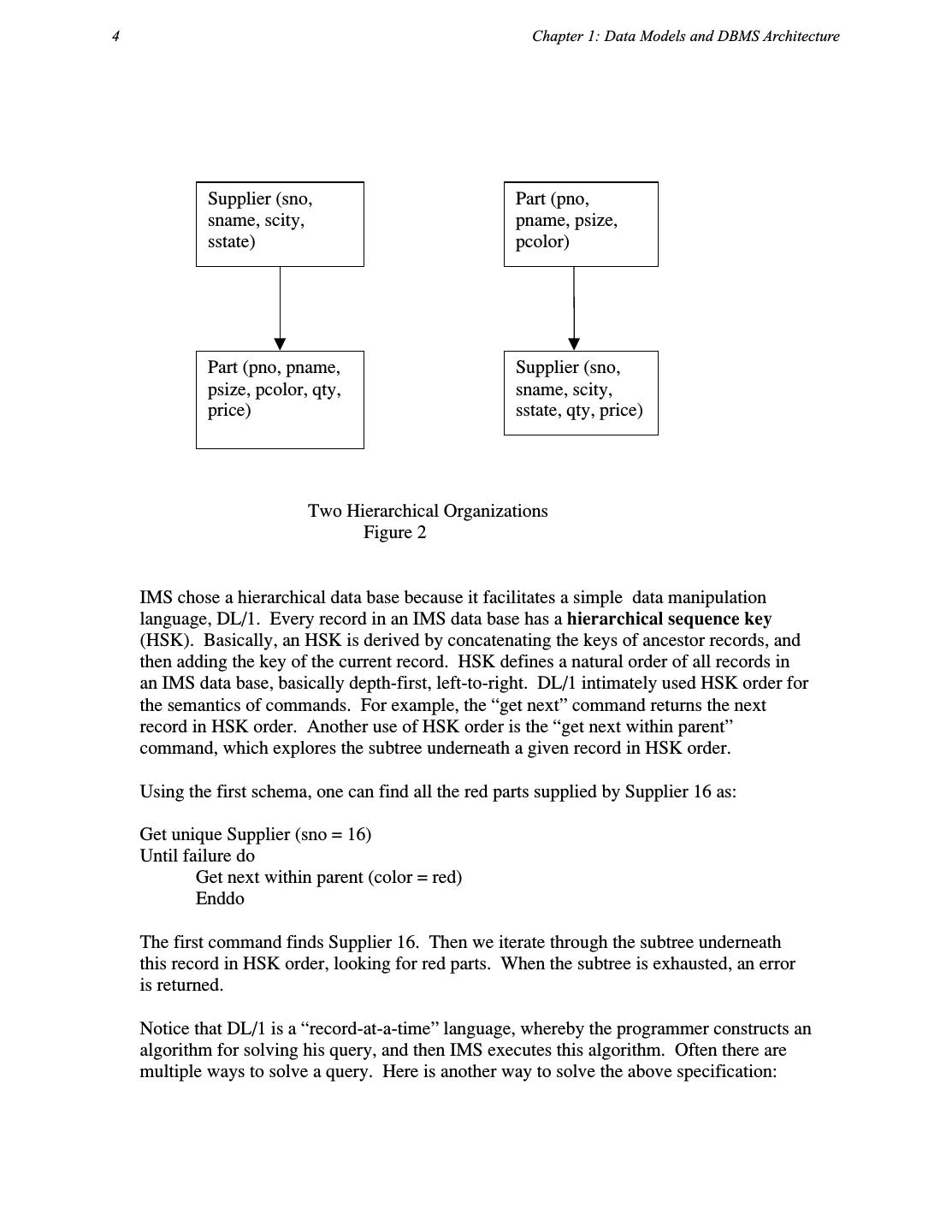
3 .4 Chapter 1: Data Models and DBMS Architecture Supplier (sno, Part (pno, sname, scity, pname, psize, sstate) pcolor) Part (pno, pname, Supplier (sno, psize, pcolor, qty, sname, scity, price) sstate, qty, price) Two Hierarchical Organizations Figure 2 IMS chose a hierarchical data base because it facilitates a simple data manipulation language, DL/1. Every record in an IMS data base has a hierarchical sequence key (HSK). Basically, an HSK is derived by concatenating the keys of ancestor records, and then adding the key of the current record. HSK defines a natural order of all records in an IMS data base, basically depth-first, left-to-right. DL/1 intimately used HSK order for the semantics of commands. For example, the “get next” command returns the next record in HSK order. Another use of HSK order is the “get next within parent” command, which explores the subtree underneath a given record in HSK order. Using the first schema, one can find all the red parts supplied by Supplier 16 as: Get unique Supplier (sno = 16) Until failure do Get next within parent (color = red) Enddo The first command finds Supplier 16. Then we iterate through the subtree underneath this record in HSK order, looking for red parts. When the subtree is exhausted, an error is returned. Notice that DL/1 is a “record-at-a-time” language, whereby the programmer constructs an algorithm for solving his query, and then IMS executes this algorithm. Often there are multiple ways to solve a query. Here is another way to solve the above specification: 

4 .What Goes Around Comes Around 5 Until failure do Get next Part (color = red) Enddo Although one might think that the second solution is clearly inferior to the first one; in fact if there is only one supplier in the data base (number 16), the second solution will outperform the first. The DL/1 programmer must make such optimization tradeoffs. IMS supported four different storage formats for hierarchical data. Basically root records can either be: Stored sequentially Indexed in a B-tree using the key of the record Hashed using the key of the record Dependent records are found from the root using either Physical sequentially Various forms of pointers. Some of the storage organizations impose restrictions on DL/1 commands. For example the purely sequential organization will not support record inserts. Hence, it is appropriate only for batch processing environments in which a change list is sorted in HSK order and then a single pass of the data base is made, the changes inserted in the correct place, and a new data base written. This is usually referred to as “old-master-new-master” processing. In addition, the storage organization that hashes root records on a key cannot support “get next”, because it has no easy way to return hashed records in HSK order. These various “quirks” in IMS are designed to avoid operations that would have impossibly bad performance. However, this decision comes at a price: One cannot freely change IMS storage organizations to tune a data base application because there is no guarantee that the DL/1 programs will continue to run. The ability of a data base application to continue to run, regardless of what tuning is performed at the physical level will be called physical data independence. Physical data independence is important because a DBMS application is not typically written all at once. As new programs are added to an application, the tuning demands may change, and better DBMS performance could be achieved by changing the storage organization. IMS has chosen to limit the amount of physical data independence that is possible. In addition, the logical requirements of an application may change over time. New record types may be added, because of new business requirements or because of new government requirements. It may also be desirable to move certain data elements from one record type to another. IMS supports a certain level of logical data independence, because DL/1 is actually defined on a logical data base, not on the actual physical data base that is stored. Hence, a DL/1 program can be written initially by defining the logical 

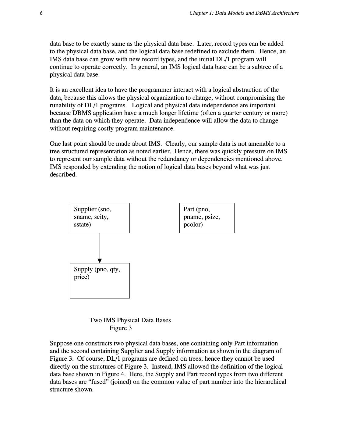
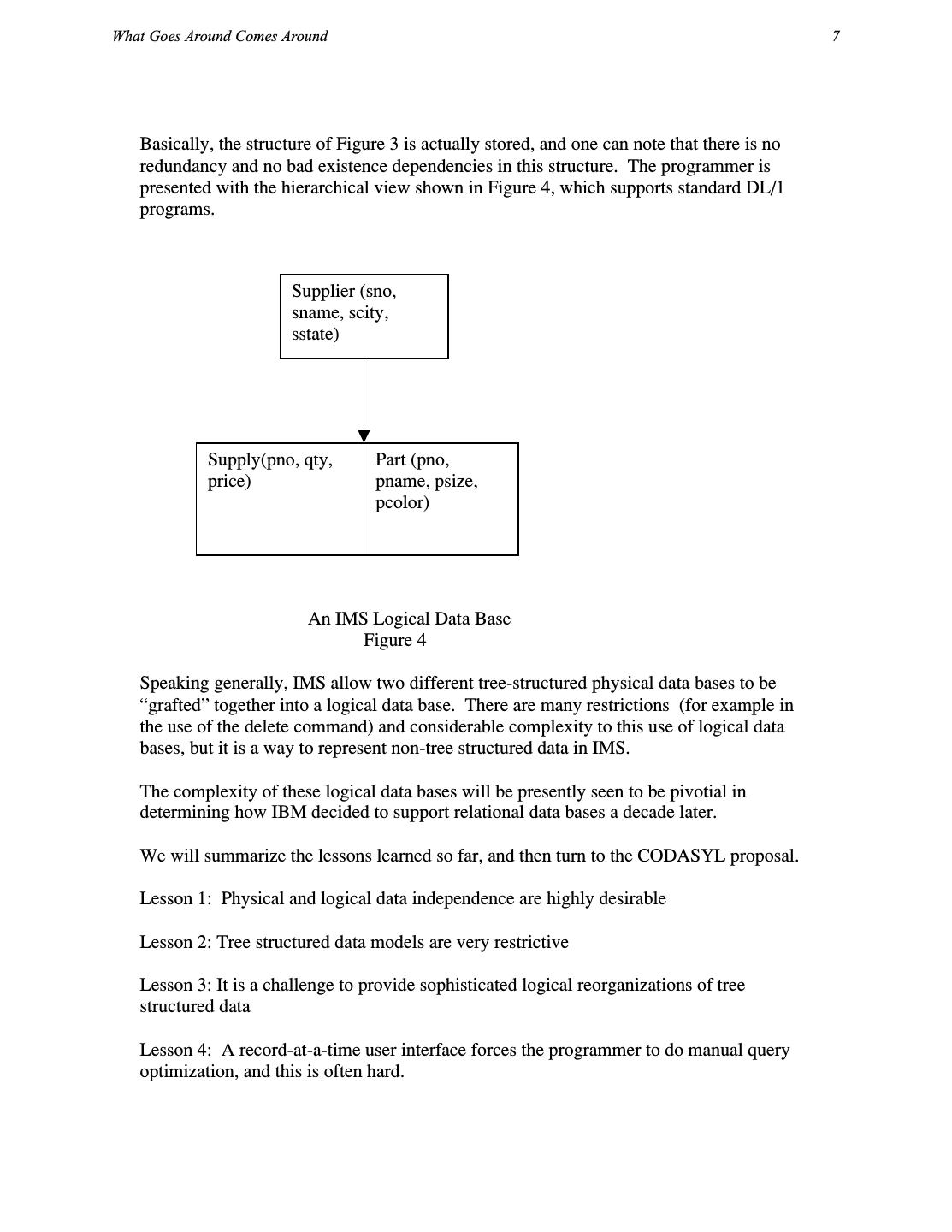
5 .6 Chapter 1: Data Models and DBMS Architecture data base to be exactly same as the physical data base. Later, record types can be added to the physical data base, and the logical data base redefined to exclude them. Hence, an IMS data base can grow with new record types, and the initial DL/1 program will continue to operate correctly. In general, an IMS logical data base can be a subtree of a physical data base. It is an excellent idea to have the programmer interact with a logical abstraction of the data, because this allows the physical organization to change, without compromising the runability of DL/1 programs. Logical and physical data independence are important because DBMS application have a much longer lifetime (often a quarter century or more) than the data on which they operate. Data independence will allow the data to change without requiring costly program maintenance. One last point should be made about IMS. Clearly, our sample data is not amenable to a tree structured representation as noted earlier. Hence, there was quickly pressure on IMS to represent our sample data without the redundancy or dependencies mentioned above. IMS responded by extending the notion of logical data bases beyond what was just described. Supplier (sno, Part (pno, sname, scity, pname, psize, sstate) pcolor) Supply (pno, qty, price) Two IMS Physical Data Bases Figure 3 Suppose one constructs two physical data bases, one containing only Part information and the second containing Supplier and Supply information as shown in the diagram of Figure 3. Of course, DL/1 programs are defined on trees; hence they cannot be used directly on the structures of Figure 3. Instead, IMS allowed the definition of the logical data base shown in Figure 4. Here, the Supply and Part record types from two different data bases are “fused” (joined) on the common value of part number into the hierarchical structure shown. 

6 .What Goes Around Comes Around 7 Basically, the structure of Figure 3 is actually stored, and one can note that there is no redundancy and no bad existence dependencies in this structure. The programmer is presented with the hierarchical view shown in Figure 4, which supports standard DL/1 programs. Supplier (sno, sname, scity, sstate) Supply(pno, qty, Part (pno, price) pname, psize, pcolor) An IMS Logical Data Base Figure 4 Speaking generally, IMS allow two different tree-structured physical data bases to be “grafted” together into a logical data base. There are many restrictions (for example in the use of the delete command) and considerable complexity to this use of logical data bases, but it is a way to represent non-tree structured data in IMS. The complexity of these logical data bases will be presently seen to be pivotial in determining how IBM decided to support relational data bases a decade later. We will summarize the lessons learned so far, and then turn to the CODASYL proposal. Lesson 1: Physical and logical data independence are highly desirable Lesson 2: Tree structured data models are very restrictive Lesson 3: It is a challenge to provide sophisticated logical reorganizations of tree structured data Lesson 4: A record-at-a-time user interface forces the programmer to do manual query optimization, and this is often hard. 

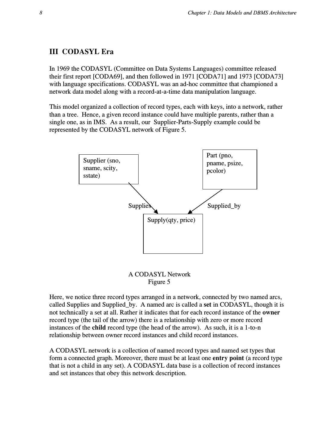
7 .8 Chapter 1: Data Models and DBMS Architecture III CODASYL Era In 1969 the CODASYL (Committee on Data Systems Languages) committee released their first report [CODA69], and then followed in 1971 [CODA71] and 1973 [CODA73] with language specifications. CODASYL was an ad-hoc committee that championed a network data model along with a record-at-a-time data manipulation language. This model organized a collection of record types, each with keys, into a network, rather than a tree. Hence, a given record instance could have multiple parents, rather than a single one, as in IMS. As a result, our Supplier-Parts-Supply example could be represented by the CODASYL network of Figure 5. Part (pno, Supplier (sno, pname, psize, sname, scity, pcolor) sstate) Supplies Supplied_by Supply(qty, price) A CODASYL Network Figure 5 Here, we notice three record types arranged in a network, connected by two named arcs, called Supplies and Supplied_by. A named arc is called a set in CODASYL, though it is not technically a set at all. Rather it indicates that for each record instance of the owner record type (the tail of the arrow) there is a relationship with zero or more record instances of the child record type (the head of the arrow). As such, it is a 1-to-n relationship between owner record instances and child record instances. A CODASYL network is a collection of named record types and named set types that form a connected graph. Moreover, there must be at least one entry point (a record type that is not a child in any set). A CODASYL data base is a collection of record instances and set instances that obey this network description. 

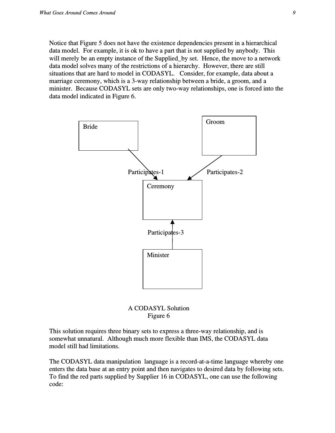
8 .What Goes Around Comes Around 9 Notice that Figure 5 does not have the existence dependencies present in a hierarchical data model. For example, it is ok to have a part that is not supplied by anybody. This will merely be an empty instance of the Supplied_by set. Hence, the move to a network data model solves many of the restrictions of a hierarchy. However, there are still situations that are hard to model in CODASYL. Consider, for example, data about a marriage ceremony, which is a 3-way relationship between a bride, a groom, and a minister. Because CODASYL sets are only two-way relationships, one is forced into the data model indicated in Figure 6. Groom Bride Participates-1 Participates-2 Ceremony Participates-3 Minister A CODASYL Solution Figure 6 This solution requires three binary sets to express a three-way relationship, and is somewhat unnatural. Although much more flexible than IMS, the CODASYL data model still had limitations. The CODASYL data manipulation language is a record-at-a-time language whereby one enters the data base at an entry point and then navigates to desired data by following sets. To find the red parts supplied by Supplier 16 in CODASYL, one can use the following code: 

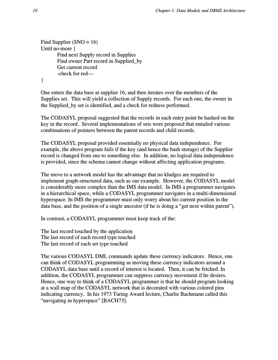
9 .10 Chapter 1: Data Models and DBMS Architecture Find Supplier (SNO = 16) Until no-more { Find next Supply record in Supplies Find owner Part record in Supplied_by Get current record -check for red— } One enters the data base at supplier 16, and then iterates over the members of the Supplies set. This will yield a collection of Supply records. For each one, the owner in the Supplied_by set is identified, and a check for redness performed. The CODASYL proposal suggested that the records in each entry point be hashed on the key in the record. Several implementations of sets were proposed that entailed various combinations of pointers between the parent records and child records. The CODASYL proposal provided essentially no physical data independence. For example, the above program fails if the key (and hence the hash storage) of the Supplier record is changed from sno to something else. In addition, no logical data independence is provided, since the schema cannot change without affecting application programs. The move to a network model has the advantage that no kludges are required to implement graph-structured data, such as our example. However, the CODASYL model is considerably more complex than the IMS data model. In IMS a programmer navigates in a hierarchical space, while a CODASYL programmer navigates in a multi-dimensional hyperspace. In IMS the programmer must only worry about his current position in the data base, and the position of a single ancestor (if he is doing a “get next within parent”). In contrast, a CODASYL programmer must keep track of the: The last record touched by the application The last record of each record type touched The last record of each set type touched The various CODASYL DML commands update these currency indicators. Hence, one can think of CODASYL programming as moving these currency indicators around a CODASYL data base until a record of interest is located. Then, it can be fetched. In addition, the CODASYL programmer can suppress currency movement if he desires. Hence, one way to think of a CODASYL programmer is that he should program looking at a wall map of the CODASYL network that is decorated with various colored pins indicating currency. In his 1973 Turing Award lecture, Charlie Bachmann called this “navigating in hyperspace” [BACH73]. 

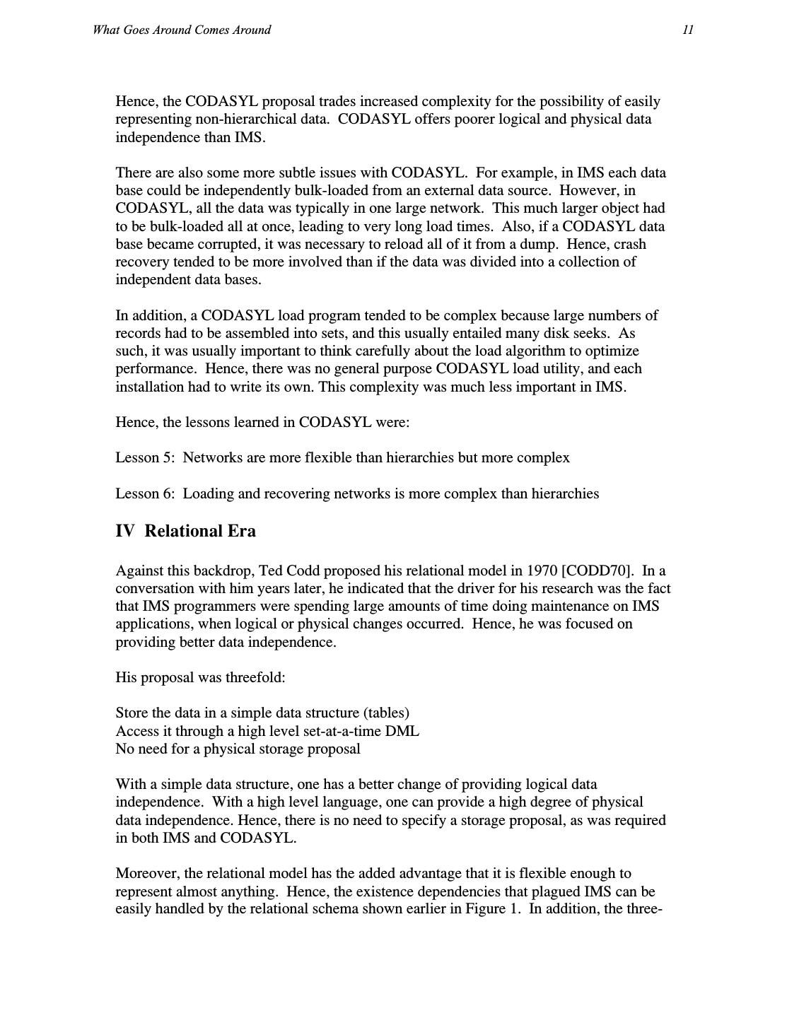
10 .What Goes Around Comes Around 11 Hence, the CODASYL proposal trades increased complexity for the possibility of easily representing non-hierarchical data. CODASYL offers poorer logical and physical data independence than IMS. There are also some more subtle issues with CODASYL. For example, in IMS each data base could be independently bulk-loaded from an external data source. However, in CODASYL, all the data was typically in one large network. This much larger object had to be bulk-loaded all at once, leading to very long load times. Also, if a CODASYL data base became corrupted, it was necessary to reload all of it from a dump. Hence, crash recovery tended to be more involved than if the data was divided into a collection of independent data bases. In addition, a CODASYL load program tended to be complex because large numbers of records had to be assembled into sets, and this usually entailed many disk seeks. As such, it was usually important to think carefully about the load algorithm to optimize performance. Hence, there was no general purpose CODASYL load utility, and each installation had to write its own. This complexity was much less important in IMS. Hence, the lessons learned in CODASYL were: Lesson 5: Networks are more flexible than hierarchies but more complex Lesson 6: Loading and recovering networks is more complex than hierarchies IV Relational Era Against this backdrop, Ted Codd proposed his relational model in 1970 [CODD70]. In a conversation with him years later, he indicated that the driver for his research was the fact that IMS programmers were spending large amounts of time doing maintenance on IMS applications, when logical or physical changes occurred. Hence, he was focused on providing better data independence. His proposal was threefold: Store the data in a simple data structure (tables) Access it through a high level set-at-a-time DML No need for a physical storage proposal With a simple data structure, one has a better change of providing logical data independence. With a high level language, one can provide a high degree of physical data independence. Hence, there is no need to specify a storage proposal, as was required in both IMS and CODASYL. Moreover, the relational model has the added advantage that it is flexible enough to represent almost anything. Hence, the existence dependencies that plagued IMS can be easily handled by the relational schema shown earlier in Figure 1. In addition, the three- 

11 .12 Chapter 1: Data Models and DBMS Architecture way marriage ceremony that was difficult in CODASYL is easily represented in the relational model as: Ceremony (bride-id, groom-id, minister-id, other-data) Codd made several (increasingly sophisticated) relational model proposals over the years [CODD79, CODDXX]. Moreover, his early DML proposals were the relational calculus (data language/alpha) [CODD71a] and the relational algebra [CODD72a]. Since Codd was originally a mathematician (and previously worked on cellular automata), his DML proposals were rigorous and formal, but not necessarily easy for mere mortals to understand. Codd’s proposal immediately touched off “the great debate”, which lasted for a good part of the 1970’s. This debate raged at SIGMOD conferences (and it predecessor SIGFIDET). On the one side, there was Ted Codd and his “followers” (mostly researchers and academics) who argued the following points: a) Nothing as complex as CODASYL can possibly be a good idea b) CODASYL does not provide acceptable data independence c) Record-at-a-time programming is too hard to optimize d) CODASYL and IMS are not flexible enough to easily represent common situations (such as marriage ceremonies) On the other side, there was Charlie Bachman and his “followers” (mostly DBMS practitioners) who argued the following: a) COBOL programmers cannot possibly understand the new-fangled relational languages b) It is impossible to implement the relational model efficiently c) CODASYL can represent tables, so what’s the big deal? The highlight (or lowlight) of this discussion was an actual debate at SIGMOD ’74 between Codd and Bachman and their respective “seconds” [RUST74]. One of us was in the audience, and it was obvious that neither side articulated their position clearly. As a result, neither side was able to hear what the other side had to say. In the next couple of years, the two camps modified their positions (more or less) as follows: Relational advocates a) Codd is a mathematician, and his languages are not the right ones. SQL [CHAM74] and QUEL [STON76] are much more user friendly. 

12 .What Goes Around Comes Around 13 b) System R [ASTR76] and INGRES [STON76] prove that efficient implementations of Codd’s ideas are possible. Moreover, query optimizers can be built that are competitive with all but the best programmers at constructing query plans. c) These systems prove that physical data independence is achievable. Moreover, relational views [STON75] offer vastly enhanced logical data independence, relative to CODASYL. d) Set-at-a-time languages offer substantial programmer productivity improvements, relative to record-at-a-time languages. CODASYL advocates a) It is possible to specify set-at-a-time network languages, such as LSL [TSIC76], that provide complete physical data independence and the possibility of better logical data independence. b) It is possible to clean up the network model [CODA78], so it is not so arcane. Hence, both camps responded to the criticisms of the other camp. The debate then died down, and attention focused on the commercial marketplace to see what would happen. Fortuitously for the relational camp, the minicomputer revolution was occurring, and VAXes were proliferating. They were an obvious target for the early commercial relational systems, such as Oracle and INGRES. Happily for the relational camp, the major CODASYL systems, such as IDMS from Culinaine Corp. were written in IBM assembler, and were not portable. Hence, the early relational systems had the VAX market to themselves. This gave them time to improve the performance of their products, and the success of the VAX market went hand-in-hand with the success of relational systems. On mainframes, a very different story was unfolding. IBM sold a derivative of System R on VM/370 and a second derivative on VSE, their low end operating system. However, neither platform was used by serious business data processing users. All the action was on MVS, the high-end operating system. Here, IBM continued to sell IMS, Cullinaine successfully sold IDMS, and relational systems were nowhere to be seen. Hence, VAXes were a relational market and mainframes were a non-relational market. At the time all serious data management was done on mainframes. This state of affairs changed abruptly in 1984, when IBM announced the upcoming release of DB/2 on MVS. In effect, IBM moved from saying that IMS was their serious DBMS to a dual data base strategy, in which both IMS and DB/2 were declared strategic. Since DB/2 was the new technology and was much easier to use, it was crystal clear to everybody who the long-term winner was going to be. 

13 .14 Chapter 1: Data Models and DBMS Architecture IBM’s signal that it was deadly serious about relational systems was a watershed moment. First, it ended once-and-for-all “the great debate”. Since IBM held vast marketplace power at the time, they effectively announced that relational systems had won and CODASYL and hierarchical systems had lost. Soon after, Cullinaine and IDMS went into a marketplace swoon. Second, they effectively declared that SQL was the de facto standard relational language. Other (substantially better) query languages, such as QUEL, were immediately dead. For a scathing critique of the semantics of SQL, consult [DATE84]. A little known fact must be discussed at this point. It would have been natural for IBM to put a relational front end on top of IMS, as shown in Figure 7. This architecture would have allowed IMS customers to continue to run IMS. New application could be written to the relational interface, providing an elegant migration path to the new technology. Hence, over time a gradual shift from DL/1 to SQL would have occurred, all the while preserving the high-performance IMS underpinnings In fact, IBM attempted to execute exactly this strategy, with a project code-named Eagle. Unfortunately, it proved too hard to implement SQL on top of the IMS notion of logical data bases, because of semantic issues. Hence, the complexity of logical data bases in IMS came back to haunt IBM many years later. As a result, IBM was forced to move to the dual data base strategy, and to declare a winner of the great debate. Old programs new programs Relational interface IMS The Architecture of Project Eagle Figure 7 In summary, the CODASL versus relational argument was ultimately settled by three events: 

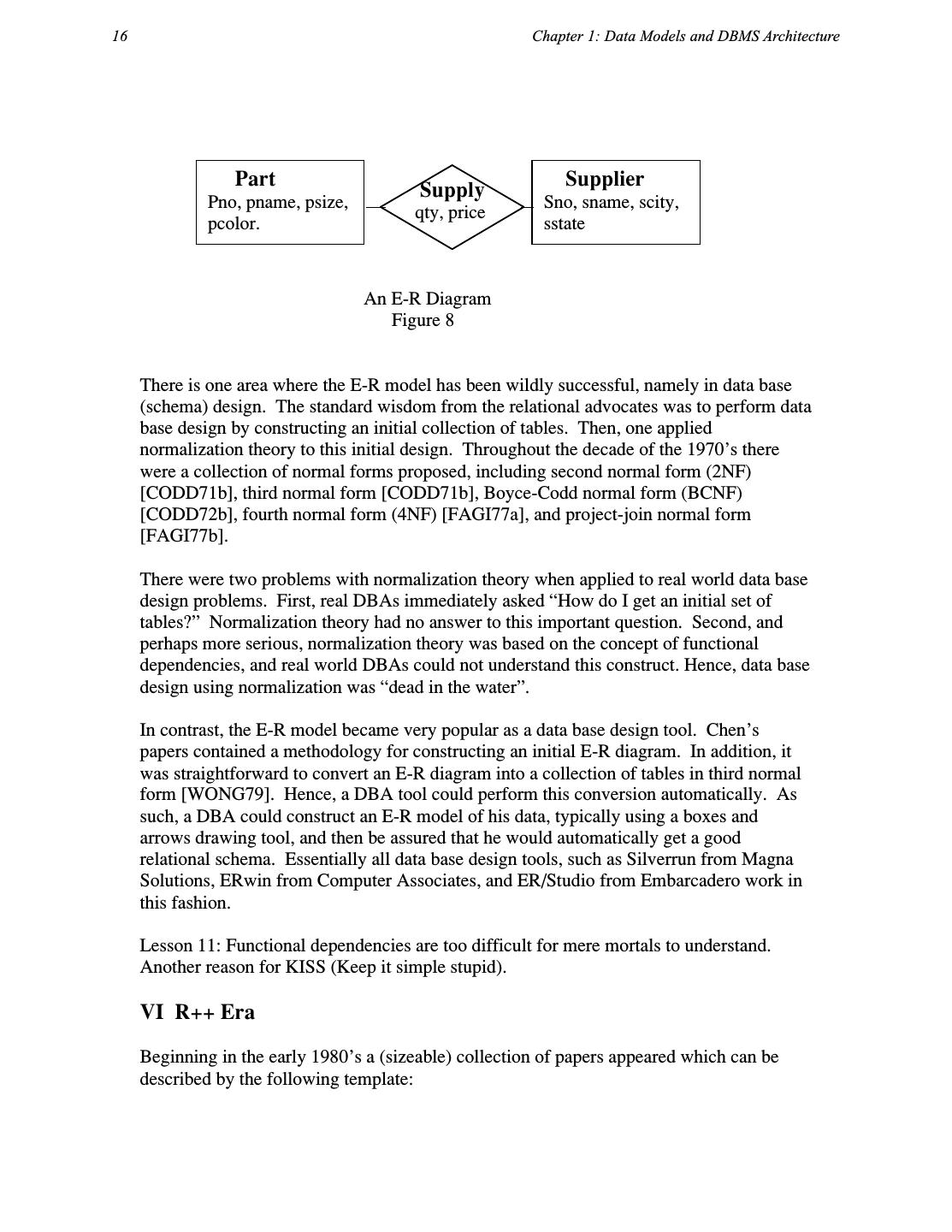
14 .What Goes Around Comes Around 15 a) the success of the VAX b) the non-portability of CODASYL engines c) the complexity of IMS logical data bases The lessons that were learned from this epoch are: Lesson 7: Set-a-time languages are good, regardless of the data model, since they offer much improved physical data independence. Lesson 8: Logical data independence is easier with a simple data model than with a complex one. Lesson 9: Technical debates are usually settled by the elephants of the marketplace, and often for reasons that have little to do with the technology. Lesson 10: Query optimizers can beat all but the best record-at-a-time DBMS application programmers. V The Entity-Relationship Era In the mid 1970’s Peter Chen proposed the entity-relationship (E-R) data model as an alternative to the relational, CODASYL and hierarchical data models [CHEN76]. Basically, he proposed that a data base be thought of a collection of instances of entities. Loosely speaking these are objects that have an existence, independent of any other entities in the data base. In our example, Supplier and Parts would be such entities. In addition, entities have attributes, which are the data elements that characterize the entity. In our example, the attributes of Part would be pno, pname, psize, and pcolor. One or more of these attributes would be designated to be unique, i.e. to be a key. Lastly, there could be relationships between entities. In our example, Supply is a relationship between the entities Part and Supplier. Relationships could be 1-to-1, 1-to-n, n-to-1 or m-to-n, depending on how the entities participate in the relationship. In our example, Suppliers can supply multiple parts, and parts can be supplied by multiple suppliers. Hence, the Supply relationship is m-to-n. Relationships can also have attributes that describe the relationship. In our example, qty and price are attributes of the relationship Supply. A popular representation for E-R models was a “boxes and arrows” notation as shown in Figure 8. The E-R model never gained acceptance as the underlying data model that is implemented by a DBMS. Perhaps the reason was that in the early days there was no query language proposed for it. Perhaps it was simply overwhelmed by the interest in the relational model in the 1970’s. Perhaps it looked too much like a “cleaned up” version of the CODASYL model. Whatever the reason, the E-R model languished in the 1970’s. 

15 .16 Chapter 1: Data Models and DBMS Architecture Part Supply Supplier Pno, pname, psize, Sno, sname, scity, qty, price pcolor. sstate An E-R Diagram Figure 8 There is one area where the E-R model has been wildly successful, namely in data base (schema) design. The standard wisdom from the relational advocates was to perform data base design by constructing an initial collection of tables. Then, one applied normalization theory to this initial design. Throughout the decade of the 1970’s there were a collection of normal forms proposed, including second normal form (2NF) [CODD71b], third normal form [CODD71b], Boyce-Codd normal form (BCNF) [CODD72b], fourth normal form (4NF) [FAGI77a], and project-join normal form [FAGI77b]. There were two problems with normalization theory when applied to real world data base design problems. First, real DBAs immediately asked “How do I get an initial set of tables?” Normalization theory had no answer to this important question. Second, and perhaps more serious, normalization theory was based on the concept of functional dependencies, and real world DBAs could not understand this construct. Hence, data base design using normalization was “dead in the water”. In contrast, the E-R model became very popular as a data base design tool. Chen’s papers contained a methodology for constructing an initial E-R diagram. In addition, it was straightforward to convert an E-R diagram into a collection of tables in third normal form [WONG79]. Hence, a DBA tool could perform this conversion automatically. As such, a DBA could construct an E-R model of his data, typically using a boxes and arrows drawing tool, and then be assured that he would automatically get a good relational schema. Essentially all data base design tools, such as Silverrun from Magna Solutions, ERwin from Computer Associates, and ER/Studio from Embarcadero work in this fashion. Lesson 11: Functional dependencies are too difficult for mere mortals to understand. Another reason for KISS (Keep it simple stupid). VI R++ Era Beginning in the early 1980’s a (sizeable) collection of papers appeared which can be described by the following template: 

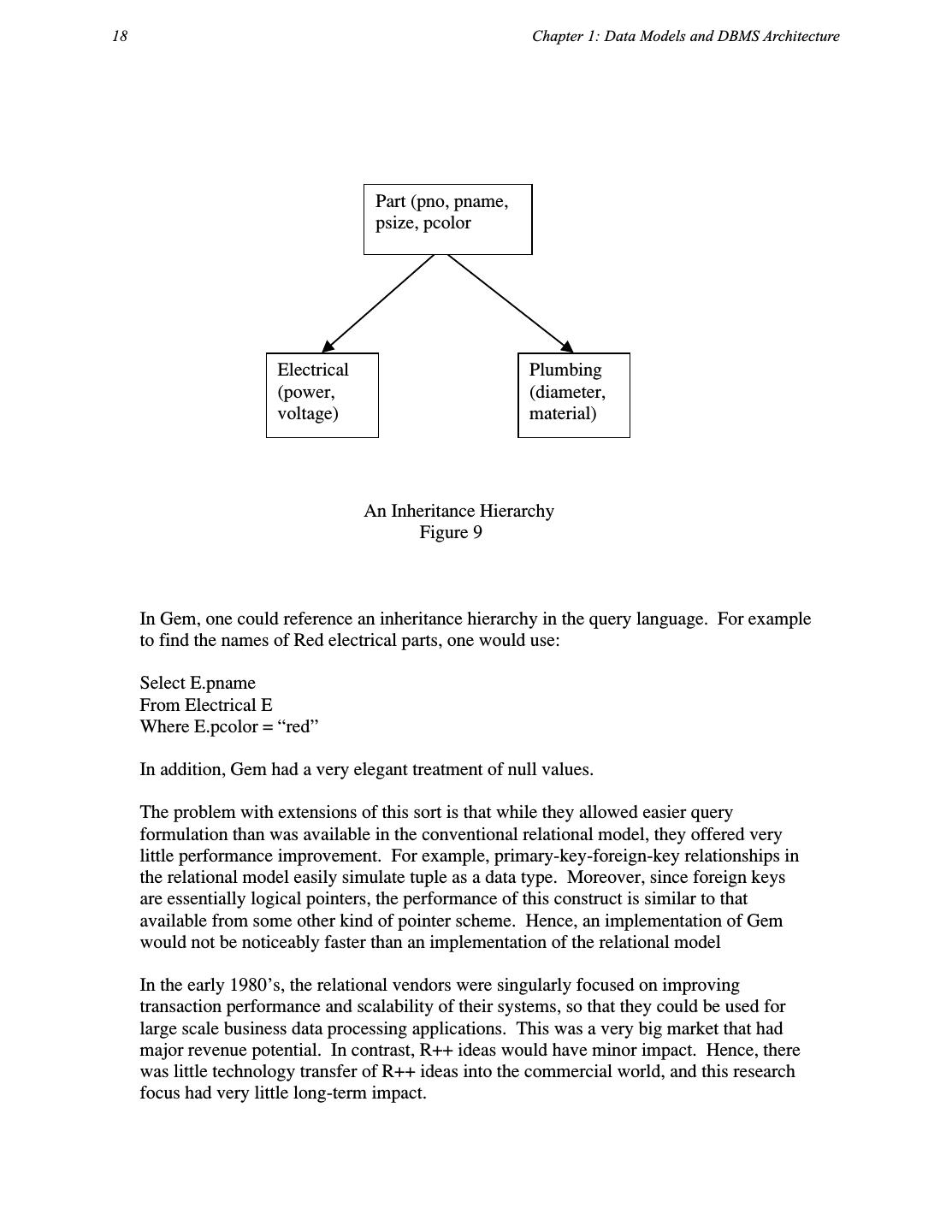
16 .What Goes Around Comes Around 17 Consider an application, call it X Try to implement X on a relational DBMS Show why the queries are difficult or why poor performance is observed Add a new “feature” to the relational model to correct the problem Many X’s were investigated including mechanical CAD [KATZ86], VLSI CAD [BATO85], text management [STON83], time [SNOD85] and computer graphics [SPON84]. This collection of papers formed “the R++ era”, as they all proposed additions to the relational model. In our opinion, probably the best of the lot was Gem [ZANI83]. Zaniolo proposed adding the following constructs to the relational model, together with corresponding query language extensions: 1) set-valued attributes. In a Parts table, it is often the case that there is an attribute, such as available_colors, which can take on a set of values. It would be nice to add a data type to the relational model to deal with sets of values. 2) aggregation (tuple-reference as a data type). In the Supply relation noted above, there are two foreign keys, sno and pno, that effectively point to tuples in other tables. It is arguably cleaner to have the Supply table have the following structure: Supply (PT, SR, qty, price) Here the data type of PT is “tuple in the Part table” and the data type of SR is “tuple in the Supplier table”. Of course, the expected implementation of these data types is via some sort of pointer. With these constructs however, we can find the suppliers who supply red parts as: Select Supply.SR.sno From Supply Where Supply.PT.pcolor = “red” This “cascaded dot” notation allowed one to query the Supply table and then effectively reference tuples in other tables. This cascaded dot notation is similar to the path expressions seen in high level network languages such as LSL. It allowed one to traverse between tables without having to specify an explicit join. 3) generalization. Suppose there are two kinds of parts in our example, say electrical parts and plumbing parts. For electrical parts, we record the power consumption and the voltage. For plumbing parts we record the diameter and the material used to make the part. This is shown pictorially in Figure 9, where we see a root part with two specializations. Each specialization inherits all of the data attributes in its ancestors. Inheritance hierarchies were put in early programming languages such as Planner [HEWI69] and Conniver [MCDO73]. The same concept has been included in more recent programming languages, such as C++. Gem merely applied this well known concept to data bases. 

17 .18 Chapter 1: Data Models and DBMS Architecture Part (pno, pname, psize, pcolor Electrical Plumbing (power, (diameter, voltage) material) An Inheritance Hierarchy Figure 9 In Gem, one could reference an inheritance hierarchy in the query language. For example to find the names of Red electrical parts, one would use: Select E.pname From Electrical E Where E.pcolor = “red” In addition, Gem had a very elegant treatment of null values. The problem with extensions of this sort is that while they allowed easier query formulation than was available in the conventional relational model, they offered very little performance improvement. For example, primary-key-foreign-key relationships in the relational model easily simulate tuple as a data type. Moreover, since foreign keys are essentially logical pointers, the performance of this construct is similar to that available from some other kind of pointer scheme. Hence, an implementation of Gem would not be noticeably faster than an implementation of the relational model In the early 1980’s, the relational vendors were singularly focused on improving transaction performance and scalability of their systems, so that they could be used for large scale business data processing applications. This was a very big market that had major revenue potential. In contrast, R++ ideas would have minor impact. Hence, there was little technology transfer of R++ ideas into the commercial world, and this research focus had very little long-term impact. 

18 .What Goes Around Comes Around 19 Lesson 12: Unless there is a big performance or functionality advantage, new constructs will go nowhere. VII The Semantic Data Model Era At around the same time, there was another school of thought with similar ideas, but a different marketing strategy. They suggested that the relational data model is “semantically impoverished”, i.e. it is incapable of easily expressing a class of data of interest. Hence, there is a need for a “post relational” data model. Post relational data models were typically called semantic data models. Examples included the work by Smith and Smith [SMIT77] and Hammer and McLeod [HAMM81]. SDM from Hammer and McLeod is arguably the more elaborate semantic data model, and we focus on its concepts in this section. SDM focuses on the notion of classes, which are a collection of records obeying the same schema. Like Gem, SDM exploited the concepts of aggregation and generalization and included a notion of sets. Aggregation is supported by allowing classes to have attributes that are records in other classes. However, SDM generalizes the aggregation construct in Gem by allowing an attribute in one class to be a set of instances of records in some class. For example, there might be two classes, Ships and Countries. The Countries class could have an attribute called Ships_registered_here, having as its value a collection of ships. The inverse attribute, country_of_registration can also be defined in SDM. In addition, classes can generalize other classes. Unlike Gem, generalization is extended to be a graph rather than just a tree. For example, Figure 10 shows a generalization graph where American_oil_tankers inherits attributes from both Oil_tankers and American_ships. This construct is often called multiple inheritance. Classes can also be the union, intersection or difference between other classes. They can also be a subclass of another class, specified by a predicate to determine membership. For example, Heavy_ships might be a subclass of Ships with weight greater than 500 tons. Lastly, a class can also be a collection of records that are grouped together for some other reason. For example Atlantic_convoy might be a collection of ships that are sailing together across the Atlantic Ocean. Lastly, classes can have class variables, for example the Ships class can have a class variable which is the number of members of the class. Most semantic data models were very complex, and were generally paper proposals. Several years after SDM was defined, Univac explored an implementation of Hammer and McLeod’s ideas. However, they quickly discovered that SQL was an intergalactic standard, and their incompatible system was not very successful in the marketplace. 

19 .20 Chapter 1: Data Models and DBMS Architecture Ships Oil_tankers American_ship American_Oil_tankers A Example of Multiple Inheritance Figure 10 In our opinion, SDMs had the same two problems that faced the R++ advocates. Like the R++ proposals, they were a lot of machinery that was easy to simulate on relational systems. Hence, there was very little leverage in the constructs being proposed. The SDM camp also faced the second issue of R++ proposals, namely that the established vendors were distracted with transaction processing performance. Hence, semantic data models had little long term influence. VIII OO Era Beginning in the mid 1980’s there was a “tidal wave” of interest in Object-oriented DBMSs (OODB). Basically, this community pointed to an “impedance mismatch” between relational data bases and languages like C++. In practice, relational data bases had their own naming systems, their own data type systems, and their own conventions for returning data as a result of a query. Whatever programming language was used alongside a relational data base also had its own version of all of these facilities. Hence, to bind an application to the data base required a conversion from “programming language speak” to “data base speak” and back. This was like “gluing an apple onto a pancake”, and was the reason for the so-called impedance mismatch. 

20 .What Goes Around Comes Around 21 For example, consider the following C++ snippet which defines a Part Structure and then allocates an Example_part. Struct Part { Int number; Char* name; Char* bigness; Char* color; } Example_part; All SQL run-time systems included mechanisms to load variables in the above Struct from values in the data base. For example to retrieve part 16 into the above Struct required the following stylized program: Define cursor P as Select * From Part Where pno = 16; Open P into Example_part Until no-more{ Fetch P (Example_part.number = pno, Example_name = pname Example_part.bigness = psize Example_part.color = pcolor) } First one defined a cursor to range over the answer to the SQL query. Then, one opened the cursor, and finally fetched a record from the cursor and bound it to programming language variables, which did not need to be the same name or type as the corresponding data base objects. If necessary, data type conversion was performed by the run-time interface. The programmer could now manipulate the Struct in the native programming language. When more than one record could result from the query, the programmer had to iterate the cursor as in the above example. It would seem to be much cleaner to integrate DBMS functionality more closely into a programming language. Specifically, one would like a persistent programming language, i.e. one where the variables in the language could represent disk-based data as well as main memory data and where data base search criteria were also language constructs. Several prototype persistent languages were developed in the late 1970’s, including Pascal-R [SCHM77], Rigel [ROWE79], and a language embedding for PL/1 [DATE76]. For example, Rigel allowed the above query to be expressed as: 

21 .22 Chapter 1: Data Models and DBMS Architecture For P in Part where P.pno = 16{ Code_to_manipulate_part } In Rigel, as in other persistent languages, variables (in this case pno) could be declared. However, they only needed to be declared once to Rigel, and not once to the language and a second time to the DBMS. In addition, the predicate p.no = 16 is part of the Rigel programming language. Lastly, one used the standard programming language iterators (in this case a For loop) to iterate over qualifying records. A persistent programming language is obviously much cleaner than a SQL embedding. However, it requires the compiler for the programming language to be extended with DBMS-oriented functionality. Since there is no programming language Esperanto, this extension must be done once per complier. Moreover, each extension will likely be unique, since C++ is quite different from, for example, APL. Unfortunately, programming language experts have consistently refused to focus on I/O in general and DBMS functionality in particular. Hence, all programming languages that we are aware of have no built-in functionality in this area. Not only does this make embedding data sublanguages tedious, but also the result is usually difficult to program and error prone. Lastly, language expertise does not get applied to important special purpose data-oriented languages, such as report writers and so-called fourth generation languages. Hence, there was no technology transfer from the persistent programming language research efforts of the 1970’s into the commercial marketplace, and ugly data- sublanguage embeddings prevailed. In the mid 1980’s there was a resurgence of interest in persistent programming languages, motivated by the popularity of C++. This research thrust was called Object-Oriented Data Bases (OODB), and focused mainly on persistent C++. Although the early work came from the research community with systems like Garden [SKAR86] and Exodus [RICH87], the primary push on OODBs came from a collection of start-ups, including Ontologic, Object Design and Versant. All built commercial systems that supported persistent C++. The general form of these systems was to support C++ as a data model. Hence, any C++ structure could be persisted. For some reason, it was popular to extend C++ with the notion of relationships, a concept borrowed directly from the Entity-Relationship data model a decade earlier. Hence, several systems extended the C++ run-time with support for this concept. Most of the OODB community decided to address engineering data bases as their target market. One typical example of this area is engineering CAD. In a CAD application, an engineer opens an engineering drawing, say for an electronic circuit, and then modifies the engineering object, tests it, or runs a power simulator on the circuit. When he is done 

22 .What Goes Around Comes Around 23 he closes the object. The general form of these applications is to open a large engineering object and then process it extensively before closing it. Historically, such objects were read into virtual memory by a load program. This program would “swizzle” a disk-based representation of the object into a virtual memory C++ object. The word “swizzle” came from the necessity of modifying any pointers in the object when loading. On disk, pointers are typically some sort of logical reference such as a foreign key, though they can also be disk pointers, for example (block-number, offset). In virtual memory, they should be virtual memory pointers. Hence, the loader had to swizzle the disk representation to a virtual memory representation. Then, the code would operate on the object, usually for a long time. When finished, an unloader would linearize the C++ data structure back into one that could persist on the disk. To address the engineering market, an implementation of persistent C++ had the following requirements: 1) no need for a declarative query language. All one needed was a way to reference large disk-based engineering objects in C++. 2) no need for fancy transaction management. This market is largely one-user-at-a- time processing large engineering objects. Rather, some sort of versioning system would be nice. 3) The run-time system had to be competitive with conventional C++ when operating on the object. In this market, the performance of an algorithm using persistent C++ had to be competitive with that available from a custom load program and conventional C++ Naturally, the OODB vendors focused on meeting these requirements. Hence, there was weak support for transactions and queries. Instead, the vendors focused on good performance for manipulating persistent C++ structures. For example, consider the following declaration: Persistent int I; And then the code snippet: I =: I+1; In conventional C++, this is a single instruction. To be competitive, incrementing a persistent variable cannot require a process switch to process a persistent object. Hence, the DBMS must run in the same address space as the application. Likewise, engineering objects must be aggressively cached in main memory, and then “lazily” written back to disk. Hence, the commercial OODBs, for example Object Design [LAMB91], had innovative architectures that achieved these objectives. 

23 .24 Chapter 1: Data Models and DBMS Architecture Unfortunately, the market for such engineering applications never got very large, and there were too many vendors competing for a “niche” market. At the present time, all of the OODB vendors have failed, or have repositioned their companies to offer something other than and OODB. For example, Object Design has renamed themselves Excelon, and is selling XML services In our opinion, there are a number of reasons for this market failure. 1) absence of leverage. The OODB vendors presented the customer with the opportunity to avoid writing a load program and an unload program. This is not a major service, and customers were not willing to pay big money for this feature. 2) No standards. All of the OODB vendor offerings were incompatible. 3) Relink the world. In anything changed, for example a C++ method that operated on persistent data, then all programs which used this method had to be relinked. This was a noticeable management problem. 4) No programming language Esperanto. If your enterprise had a single application not written in C++ that needed to access persistent data, then you could not use one of the OODB products. Of course, the OODB products were not designed to work on business data processing applications. Not only did they lack strong transaction and query systems but also they ran in the same address space as the application. This meant that the application could freely manipulate all disk-based data, and no data protection was possible. Protection and authorization is important in the business data processing market. In addition, OODBs were clearly a throw back to the CODASYL days, i.e. a low-level record at a time language with the programmer coding the query optimization algorithm. As a result, these products had essentially no penetration in this very large market. There was one company, O2, that had a different business plan. O2 supported an object- oriented data model, but it was not C++. Also, they embedded a high level declarative language called OQL into a programming language. Hence, they proposed what amounted to a semantic data model with a declarative query language, but marketed it as an OODB. Also, they focused on business data processing, not on the engineering application space. Unfortunately for O2, there is a saying that “as goes the United States goes the rest of the world”. This means that new products must make it in North America, and that the rest of the world watches the US for market acceptance. O2 was a French company, spun out of Inria by Francois Bancilhon. It was difficult for O2 to get market traction in Europe with an advanced product, because of the above adage. Hence, O2 realized they had to attack the US market, and moved to the United States rather late in the game. By then, it was simply too late, and the OODB era was on a downward spiral. It is interesting to conjecture about the marketplace chances of O2 if they had started initially in the USA with sophisticated US venture capital backing. Lesson 13: Packages will not sell to users unless they are in “major pain” 

24 .What Goes Around Comes Around 25 Lesson 14: Persistent languages will go nowhere without the support of the programming language community. IX The Object-Relational Era The Object-Relational (OR) era was motivated by a very simple problem. In the early days of INGRES, the team had been interested in geographic information systems (GIS) and had suggested mechanisms for their support [GO75]. Around 1982, the following simple GIS issue was haunting the INGRES research team. Suppose one wants to store geographic positions in a data base. For example, one might want to store the location of a collection of intersections as: Intersections (I-id, long, lat, other-data) Here, we require storing geographic points (long, lat) in a data base. Then, if we want to find all the intersections within a bounding rectangle, (X0, Y0, X1, Y1), then the SQL query is: Select I-id From Intersections Where X0 < long < X1 and Y0 < lat < Y1 Unfortunately, this is a two dimensional search, and the B-trees in INGRES are a one- dimensional access method. One-dimensional access methods do not do two- dimensional searches efficiently, so there is no way in a relational system for this query to run fast. More troubling was the “notify parcel owners” problem. Whenever there is request for a variance to the zoning laws for a parcel of land in California, there must be a public hearing, and all property owners within a certain distance must be notified. Suppose one assumes that all parcels are rectangles, and they are stored in the following table. Parcel (P-id, Xmin, Xmax, Ymin, Ymax) Then, one must enlarge the parcel in question by the correct number of feet, creating a “super rectangle” with co-ordinates X0, X1, Y0, Y1. All property owners whose parcels intersect this super rectangle must be notified, and the most efficient query to do this task is: Select P-id From Parcel Where Xmax > X0 and Ymax > Y0 and Xmin < X1 and Ymax < Y1 

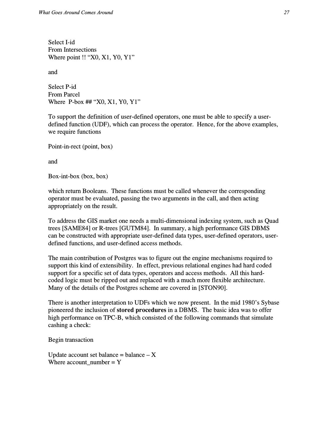
25 .26 Chapter 1: Data Models and DBMS Architecture Again, there is no way to execute this query efficiency with a B-tree access method. Moreover, it takes a moment to convince oneself that this query is correct, and there are several other less efficient representations. In summary, simple GIS queries are difficult to express in SQL, and they execute on standard B-trees with unreasonably bad performance. The following observation motivates the OR proposal. Early relational systems supported integers, floats, and character strings, along with the obvious operators, primarily because these were the data types of IMS, which was the early competition. IMS chose these data types because that was what the business data processing market wanted, and that was their market focus. Relational systems also chose B-trees because these facilitate the searches that are common in business data processing. Later relational systems expanded the collection of business data processing data types to include date, time and money. More recently, packed decimal and blobs have been added. In other markets, such as GIS, these are not the correct types, and B-trees are not the correct access method. Hence, to address any given market, one needs data types and access methods appropriate to the market. Since there may be many other markets one would want to address, it is inappropriate to “hard wire” a specific collection of data types and indexing strategies. Rather a sophisticated user should be able to add his own; i.e. to customize a DBMS to his particular needs. Such customization is also helpful in business data processing, since one or more new data types appears to be needed every decade. As a result, the OR proposal added user-defined data types, user-defined operators, user-defined functions, and user-defined access methods to a SQL engine. The major OR research prototype was Postgres [STON86]. Applying the OR methodology to GIS, one merely adds geographic points and geographic boxes as data types. With these data types, the above tables above can be expressed as: Intersections (I-id, point, other-data) Parcel (P-id, P-box) Of course, one must also have SQL operators appropriate to each data type. For our simple application, these are !! (point in rectangle) and ## (box intersects box). The two queries now become 

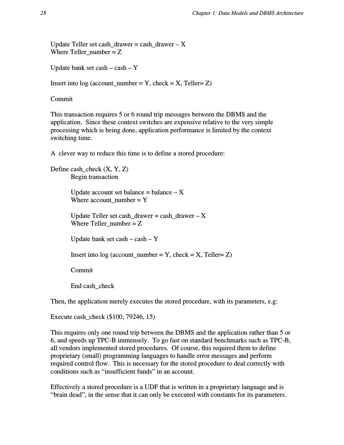
26 .What Goes Around Comes Around 27 Select I-id From Intersections Where point !! “X0, X1, Y0, Y1” and Select P-id From Parcel Where P-box ## “X0, X1, Y0, Y1” To support the definition of user-defined operators, one must be able to specify a user- defined function (UDF), which can process the operator. Hence, for the above examples, we require functions Point-in-rect (point, box) and Box-int-box (box, box) which return Booleans. These functions must be called whenever the corresponding operator must be evaluated, passing the two arguments in the call, and then acting appropriately on the result. To address the GIS market one needs a multi-dimensional indexing system, such as Quad trees [SAME84] or R-trees [GUTM84]. In summary, a high performance GIS DBMS can be constructed with appropriate user-defined data types, user-defined operators, user- defined functions, and user-defined access methods. The main contribution of Postgres was to figure out the engine mechanisms required to support this kind of extensibility. In effect, previous relational engines had hard coded support for a specific set of data types, operators and access methods. All this hard- coded logic must be ripped out and replaced with a much more flexible architecture. Many of the details of the Postgres scheme are covered in [STON90]. There is another interpretation to UDFs which we now present. In the mid 1980’s Sybase pioneered the inclusion of stored procedures in a DBMS. The basic idea was to offer high performance on TPC-B, which consisted of the following commands that simulate cashing a check: Begin transaction Update account set balance = balance – X Where account_number = Y 

27 .28 Chapter 1: Data Models and DBMS Architecture Update Teller set cash_drawer = cash_drawer – X Where Teller_number = Z Update bank set cash – cash – Y Insert into log (account_number = Y, check = X, Teller= Z) Commit This transaction requires 5 or 6 round trip messages between the DBMS and the application. Since these context switches are expensive relative to the very simple processing which is being done, application performance is limited by the context switching time. A clever way to reduce this time is to define a stored procedure: Define cash_check (X, Y, Z) Begin transaction Update account set balance = balance – X Where account_number = Y Update Teller set cash_drawer = cash_drawer – X Where Teller_number = Z Update bank set cash – cash – Y Insert into log (account_number = Y, check = X, Teller= Z) Commit End cash_check Then, the application merely executes the stored procedure, with its parameters, e.g: Execute cash_check ($100, 79246, 15) This requires only one round trip between the DBMS and the application rather than 5 or 6, and speeds up TPC-B immensely. To go fast on standard benchmarks such as TPC-B, all vendors implemented stored procedures. Of course, this required them to define proprietary (small) programming languages to handle error messages and perform required control flow. This is necessary for the stored procedure to deal correctly with conditions such as “insufficient funds” in an account. Effectively a stored procedure is a UDF that is written in a proprietary language and is “brain dead”, in the sense that it can only be executed with constants for its parameters. 

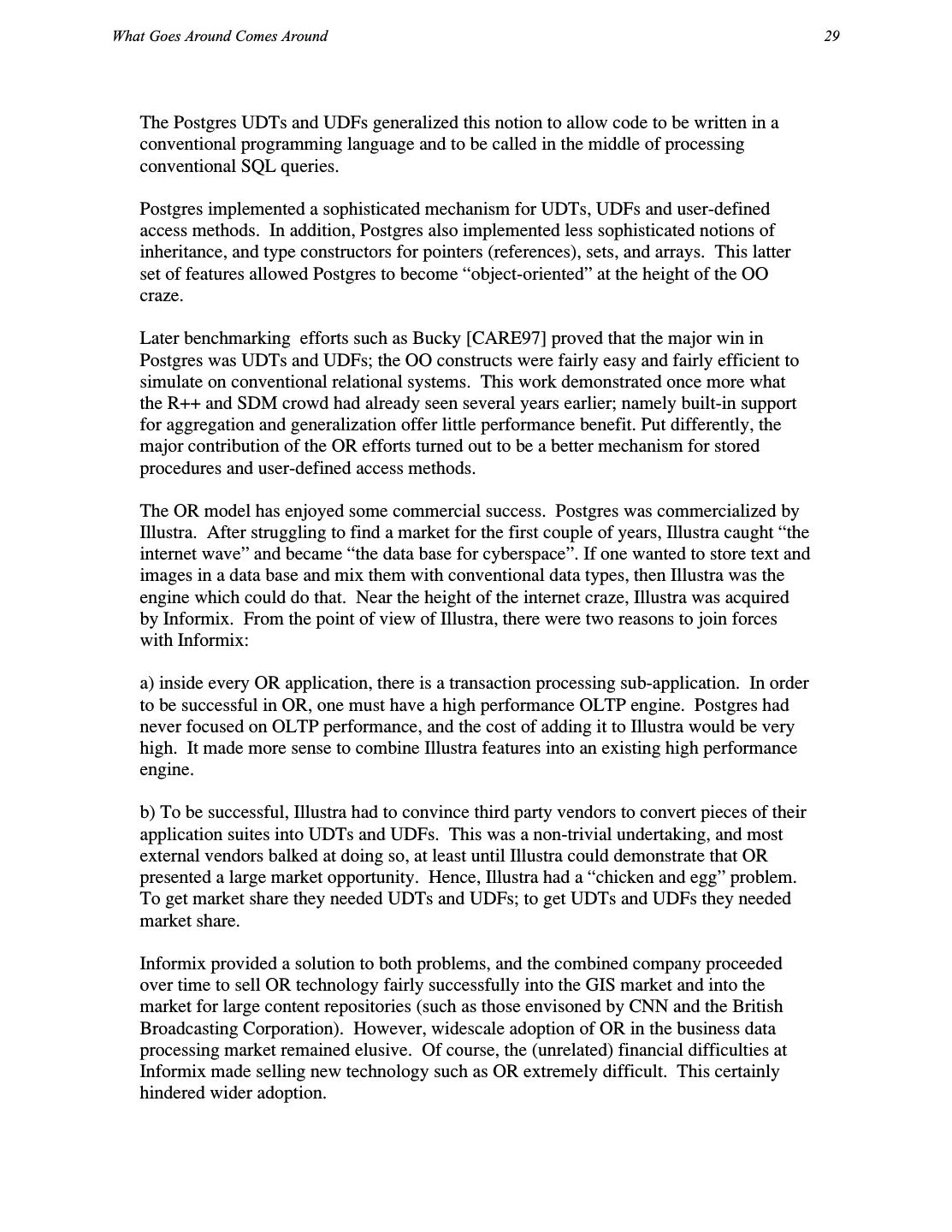
28 .What Goes Around Comes Around 29 The Postgres UDTs and UDFs generalized this notion to allow code to be written in a conventional programming language and to be called in the middle of processing conventional SQL queries. Postgres implemented a sophisticated mechanism for UDTs, UDFs and user-defined access methods. In addition, Postgres also implemented less sophisticated notions of inheritance, and type constructors for pointers (references), sets, and arrays. This latter set of features allowed Postgres to become “object-oriented” at the height of the OO craze. Later benchmarking efforts such as Bucky [CARE97] proved that the major win in Postgres was UDTs and UDFs; the OO constructs were fairly easy and fairly efficient to simulate on conventional relational systems. This work demonstrated once more what the R++ and SDM crowd had already seen several years earlier; namely built-in support for aggregation and generalization offer little performance benefit. Put differently, the major contribution of the OR efforts turned out to be a better mechanism for stored procedures and user-defined access methods. The OR model has enjoyed some commercial success. Postgres was commercialized by Illustra. After struggling to find a market for the first couple of years, Illustra caught “the internet wave” and became “the data base for cyberspace”. If one wanted to store text and images in a data base and mix them with conventional data types, then Illustra was the engine which could do that. Near the height of the internet craze, Illustra was acquired by Informix. From the point of view of Illustra, there were two reasons to join forces with Informix: a) inside every OR application, there is a transaction processing sub-application. In order to be successful in OR, one must have a high performance OLTP engine. Postgres had never focused on OLTP performance, and the cost of adding it to Illustra would be very high. It made more sense to combine Illustra features into an existing high performance engine. b) To be successful, Illustra had to convince third party vendors to convert pieces of their application suites into UDTs and UDFs. This was a non-trivial undertaking, and most external vendors balked at doing so, at least until Illustra could demonstrate that OR presented a large market opportunity. Hence, Illustra had a “chicken and egg” problem. To get market share they needed UDTs and UDFs; to get UDTs and UDFs they needed market share. Informix provided a solution to both problems, and the combined company proceeded over time to sell OR technology fairly successfully into the GIS market and into the market for large content repositories (such as those envisoned by CNN and the British Broadcasting Corporation). However, widescale adoption of OR in the business data processing market remained elusive. Of course, the (unrelated) financial difficulties at Informix made selling new technology such as OR extremely difficult. This certainly hindered wider adoption. 

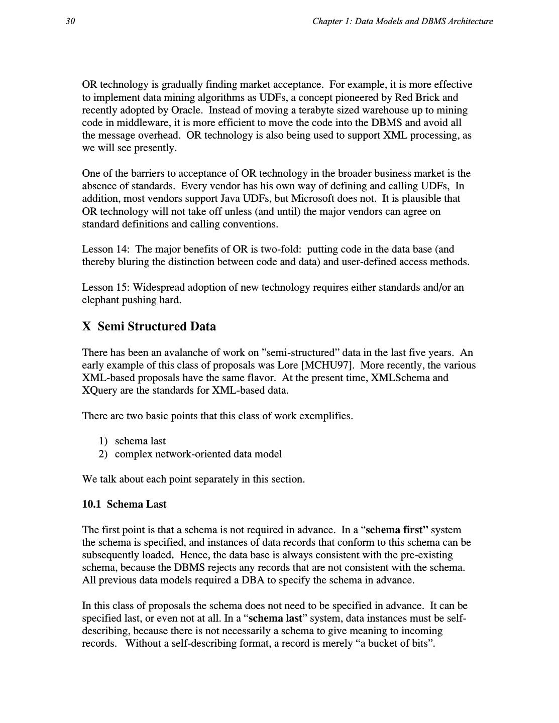
29 .30 Chapter 1: Data Models and DBMS Architecture OR technology is gradually finding market acceptance. For example, it is more effective to implement data mining algorithms as UDFs, a concept pioneered by Red Brick and recently adopted by Oracle. Instead of moving a terabyte sized warehouse up to mining code in middleware, it is more efficient to move the code into the DBMS and avoid all the message overhead. OR technology is also being used to support XML processing, as we will see presently. One of the barriers to acceptance of OR technology in the broader business market is the absence of standards. Every vendor has his own way of defining and calling UDFs, In addition, most vendors support Java UDFs, but Microsoft does not. It is plausible that OR technology will not take off unless (and until) the major vendors can agree on standard definitions and calling conventions. Lesson 14: The major benefits of OR is two-fold: putting code in the data base (and thereby bluring the distinction between code and data) and user-defined access methods. Lesson 15: Widespread adoption of new technology requires either standards and/or an elephant pushing hard. X Semi Structured Data There has been an avalanche of work on ”semi-structured” data in the last five years. An early example of this class of proposals was Lore [MCHU97]. More recently, the various XML-based proposals have the same flavor. At the present time, XMLSchema and XQuery are the standards for XML-based data. There are two basic points that this class of work exemplifies. 1) schema last 2) complex network-oriented data model We talk about each point separately in this section. 10.1 Schema Last The first point is that a schema is not required in advance. In a “schema first” system the schema is specified, and instances of data records that conform to this schema can be subsequently loaded. Hence, the data base is always consistent with the pre-existing schema, because the DBMS rejects any records that are not consistent with the schema. All previous data models required a DBA to specify the schema in advance. In this class of proposals the schema does not need to be specified in advance. It can be specified last, or even not at all. In a “schema last” system, data instances must be self- describing, because there is not necessarily a schema to give meaning to incoming records. Without a self-describing format, a record is merely “a bucket of bits”.