视觉特征检测器

下载 0

乐乐

发布于

3295

人观看

#信息技术

在我们进行图像捕捉时，你需要注意什么呢？是全部包含还是需要有局部的不变特征来突出图像的特征呢？本章节就此做了介绍，介绍了局部不变的特征，以及在重要部分进行定位的一款检测器--harris 特征视觉检测器的作用等。

展开查看详情

1 . Lecture 6: Finding Features (part 1/2) Professor Fei-‐Fei Li Stanford Vision Lab Fei-Fei Li! Lecture 6 - !1 2-‐Oct-‐14

2 . What we will learn today? •  Local invariant features –  MoHvaHon –  Requirements, invariances •  Keypoint localizaHon –  Harris corner detector •  Scale invariant region selecHon –  AutomaHc scale selecHon Next lecture (#7) –  Diﬀerence-‐of-‐Gaussian (DoG) detector •  SIFT: an image region descriptor Fei-Fei Li! Lecture 6 - !2 2-‐Oct-‐14

3 . What we will learn today? •  Local invariant features –  MoHvaHon –  Requirements, invariances •  Keypoint localizaHon –  Harris corner detector •  Scale invariant region selecHon –  AutomaHc scale selecHon –  Diﬀerence-‐of-‐Gaussian (DoG) detector SIFT: • Some an image background reading: region descriptor Rick Szeliski, Chapter 14.1.1; David Lowe, IJCV 2004 Fei-Fei Li! Lecture 6 - !3 2-‐Oct-‐14

4 . Image matching: a challenging problem Fei-Fei Li! Lecture 6 - !4 2-‐Oct-‐14

5 . Image matching: a challenging problem Slide credit: Steve Seitz by Diva Sian by swashford Fei-Fei Li! Lecture 6 - !5 2-‐Oct-‐14

6 . Harder Case Slide credit: Steve Seitz by Diva Sian by scgbt Fei-Fei Li! Lecture 6 - !6 2-‐Oct-‐14

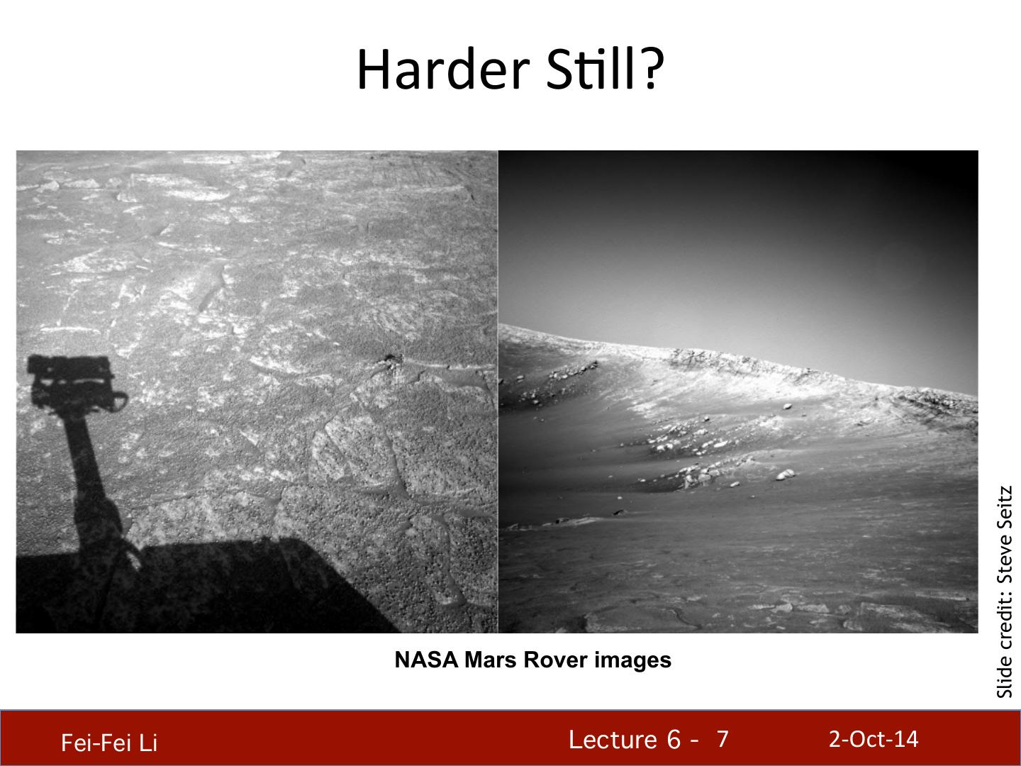
7 . Harder SHll? Slide credit: Steve Seitz NASA Mars Rover images Fei-Fei Li! Lecture 6 - !7 2-‐Oct-‐14

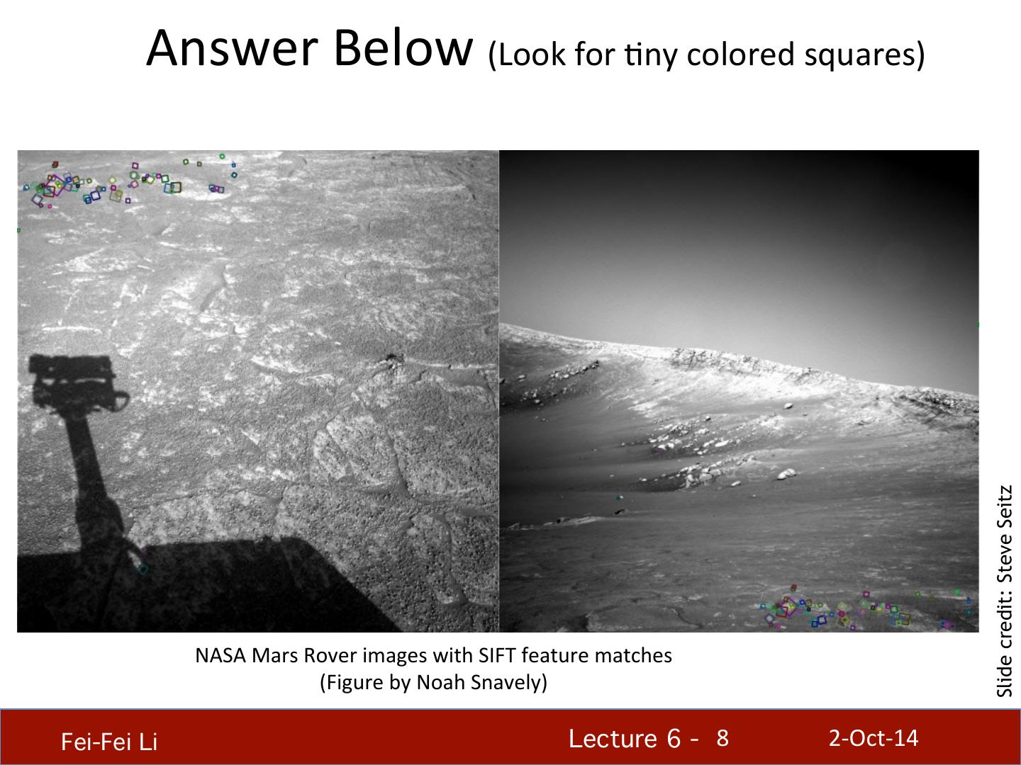
8 . Answer Below (Look for Hny colored squares) Slide credit: Steve Seitz NASA Mars Rover images with SIFT feature matches (Figure by Noah Snavely) Fei-Fei Li! Lecture 6 - !8 2-‐Oct-‐14

9 . MoHvaHon for using local features •  Global representaHons have major limitaHons •  Instead, describe and match only local regions •  Increased robustness to –  Occlusions –  ArHculaHon d dq φ φ θq θ –  Intra-‐category variaHons Fei-Fei Li! Lecture 6 - !9 2-‐Oct-‐14

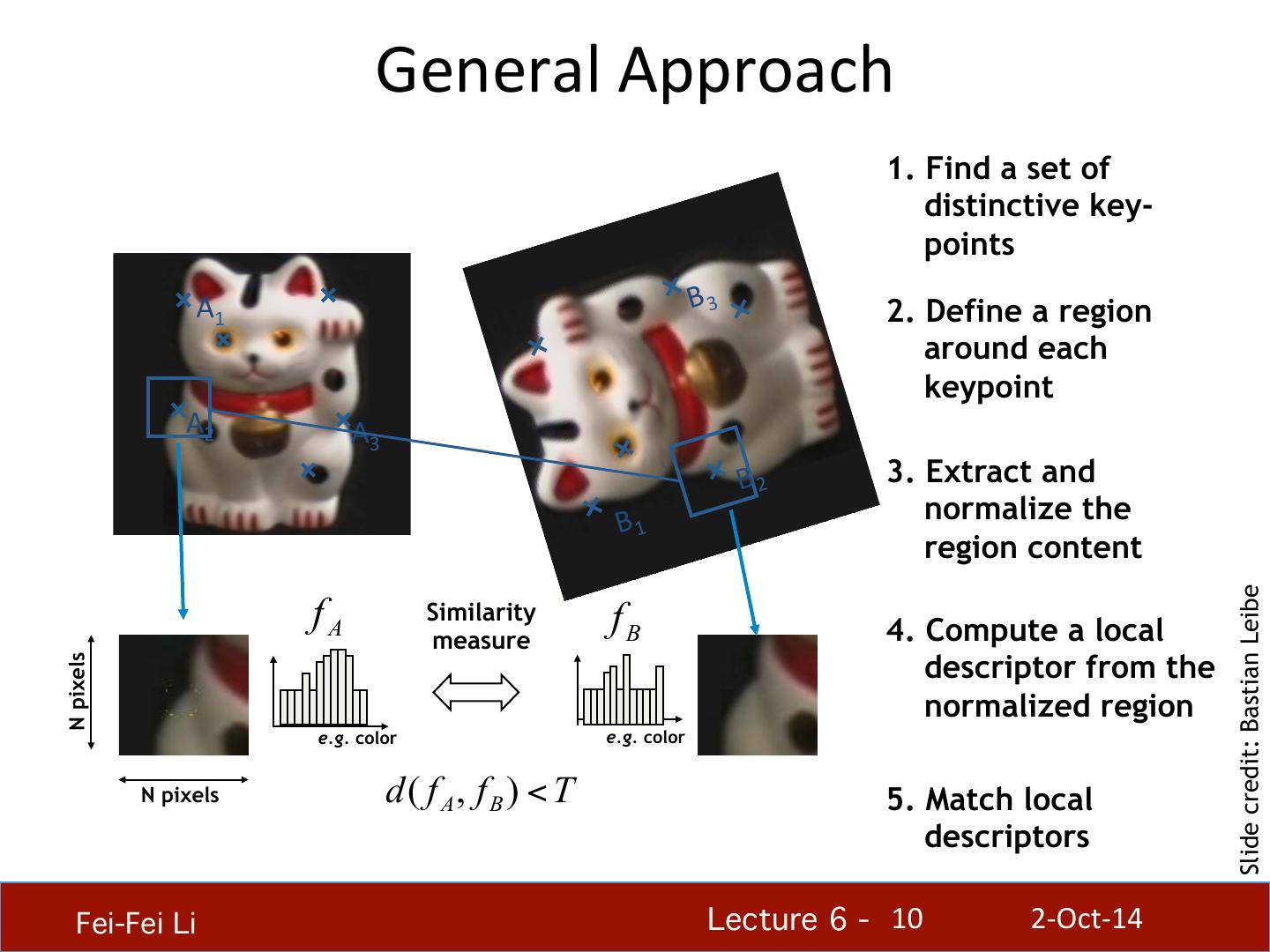
10 . General Approach 1. Find a set of distinctive key- points A1 B 3 2. Define a region around each keypoint A2 A3 B 2 3. Extract and B 1 normalize the region content Slide credit: Bastian Leibe fA Similarity fB 4. Compute a local measure descriptor from the N pixels normalized region e.g. color e.g. color N pixels d( f A, fB ) < T 5. Match local descriptors Fei-Fei Li! Lecture 6 - !10 2-‐Oct-‐14

11 . Common Requirements •  Problem 1: –  Detect the same point independently in both images Slide credit: Darya Frolova, Denis Simakov No chance to match! We need a repeatable detector! Fei-Fei Li! Lecture 6 - !11 2-‐Oct-‐14

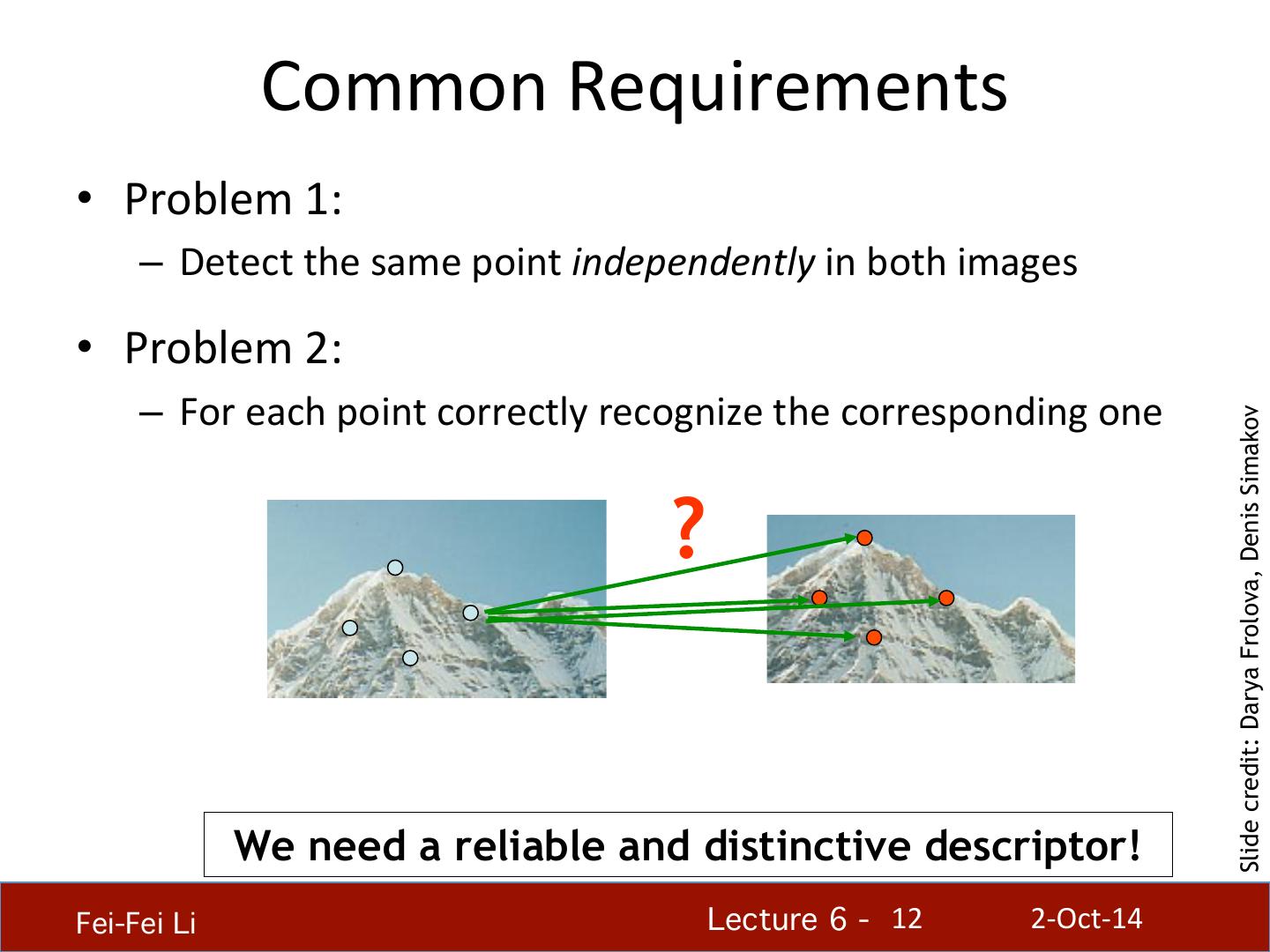
12 . Common Requirements •  Problem 1: –  Detect the same point independently in both images •  Problem 2: –  For each point correctly recognize the corresponding one Slide credit: Darya Frolova, Denis Simakov ? We need a reliable and distinctive descriptor! Fei-Fei Li! Lecture 6 - !12 2-‐Oct-‐14

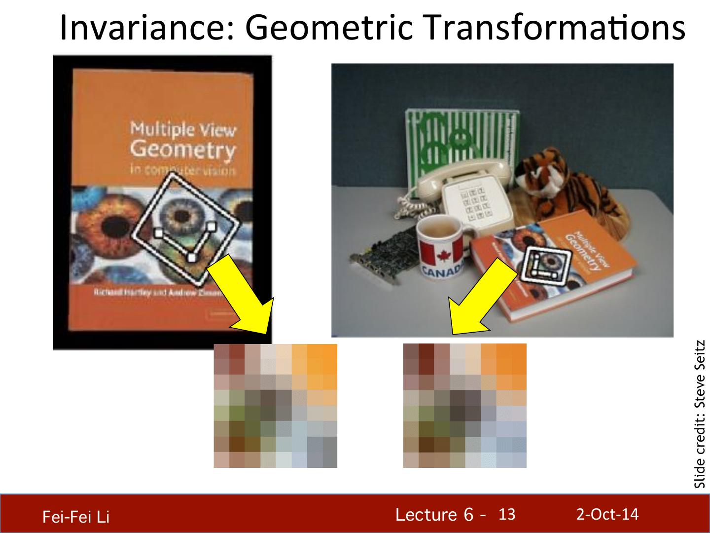
13 . Invariance: Geometric TransformaHons Slide credit: Steve Seitz Fei-Fei Li! Lecture 6 - !13 2-‐Oct-‐14

14 . Levels of Geometric Invariance Slide credit: Bastian Leibe CS131 CS231a Fei-Fei Li! Lecture 6 - !14 2-‐Oct-‐14

15 .Invariance: Photometric TransformaHons Slide credit: Tinne Tuytelaars •  Ofen modeled as a linear transformaHon: –  Scaling + Oﬀset Fei-Fei Li! Lecture 6 - !15 2-‐Oct-‐14

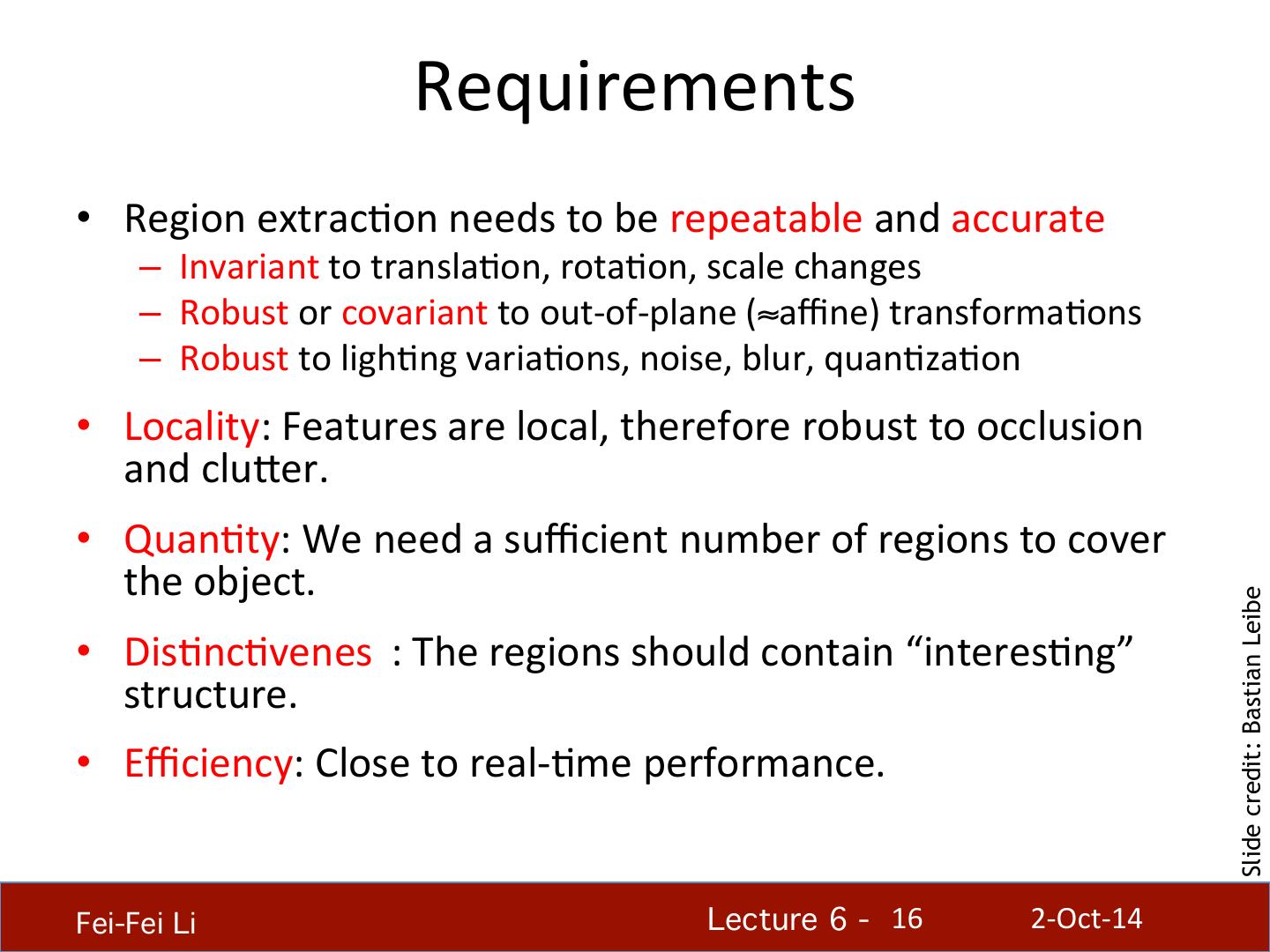
16 . Requirements •  Region extracHon needs to be repeatable and accurate –  Invariant to translaHon, rotaHon, scale changes –  Robust or covariant to out-‐of-‐plane (≈aﬃne) transformaHons –  Robust to lighHng variaHons, noise, blur, quanHzaHon •  Locality: Features are local, therefore robust to occlusion and cluier. •  QuanHty: We need a suﬃcient number of regions to cover the object. Slide credit: Bastian Leibe •  DisHncHveness: The regions should contain “interesHng” structure. •  Eﬃciency: Close to real-‐Hme performance. Fei-Fei Li! Lecture 6 - !16 2-‐Oct-‐14

17 . Many ExisHng Detectors Available •  Hessian & Harris [Beaudet ‘78], [Harris ‘88] •  Laplacian, DoG [Lindeberg ‘98], [Lowe ‘99] •  Harris-‐/Hessian-‐Laplace [Mikolajczyk & Schmid ‘01] •  Harris-‐/Hessian-‐Aﬃne [Mikolajczyk & Schmid ‘04] •  EBR and IBR [Tuytelaars & Van Gool ‘04] •  MSER [Matas ‘02] •  Salient Regions [Kadir & Brady ‘01] Slide credit: Bastian Leibe •  Others… •  Those detectors have become a basic building block for many recent applica8ons in Computer Vision. Fei-Fei Li! Lecture 6 - !17 2-‐Oct-‐14

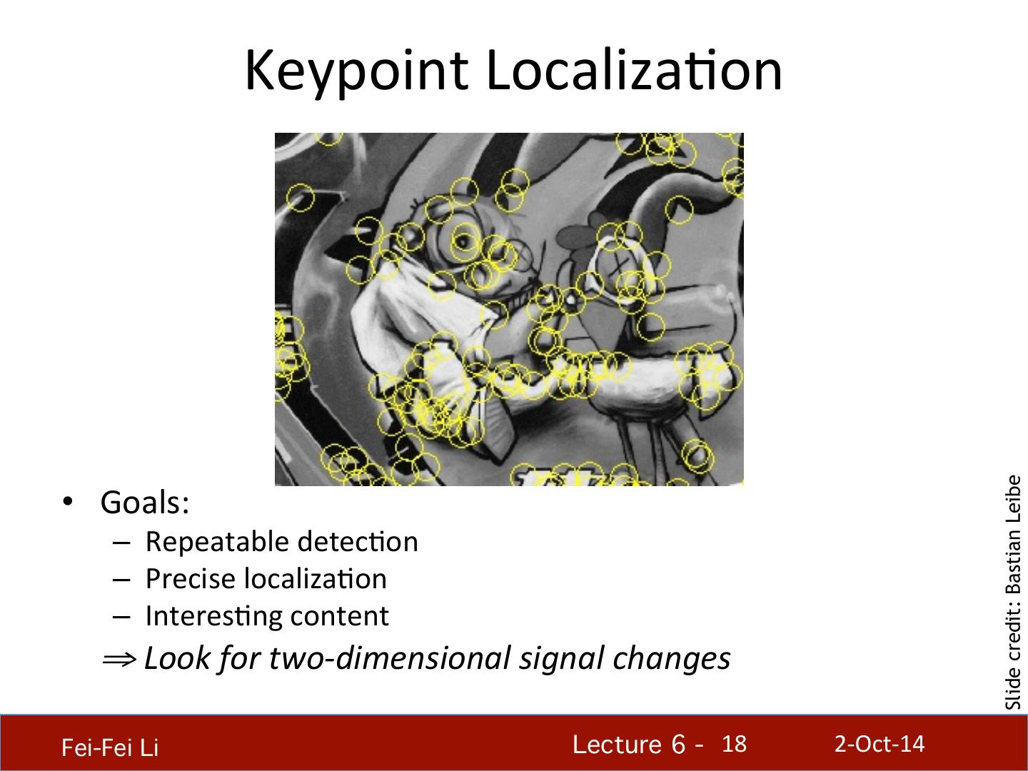
18 . Keypoint LocalizaHon Slide credit: Bastian Leibe •  Goals: –  Repeatable detecHon –  Precise localizaHon –  InteresHng content ⇒ Look for two-‐dimensional signal changes Fei-Fei Li! Lecture 6 - !18 2-‐Oct-‐14

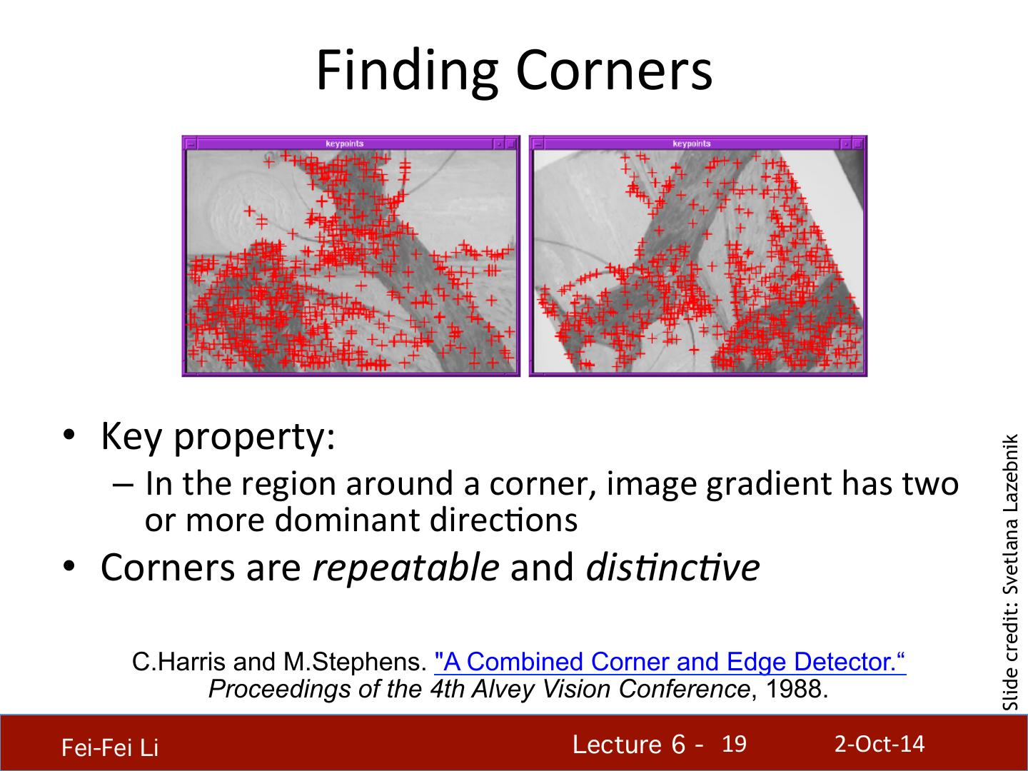
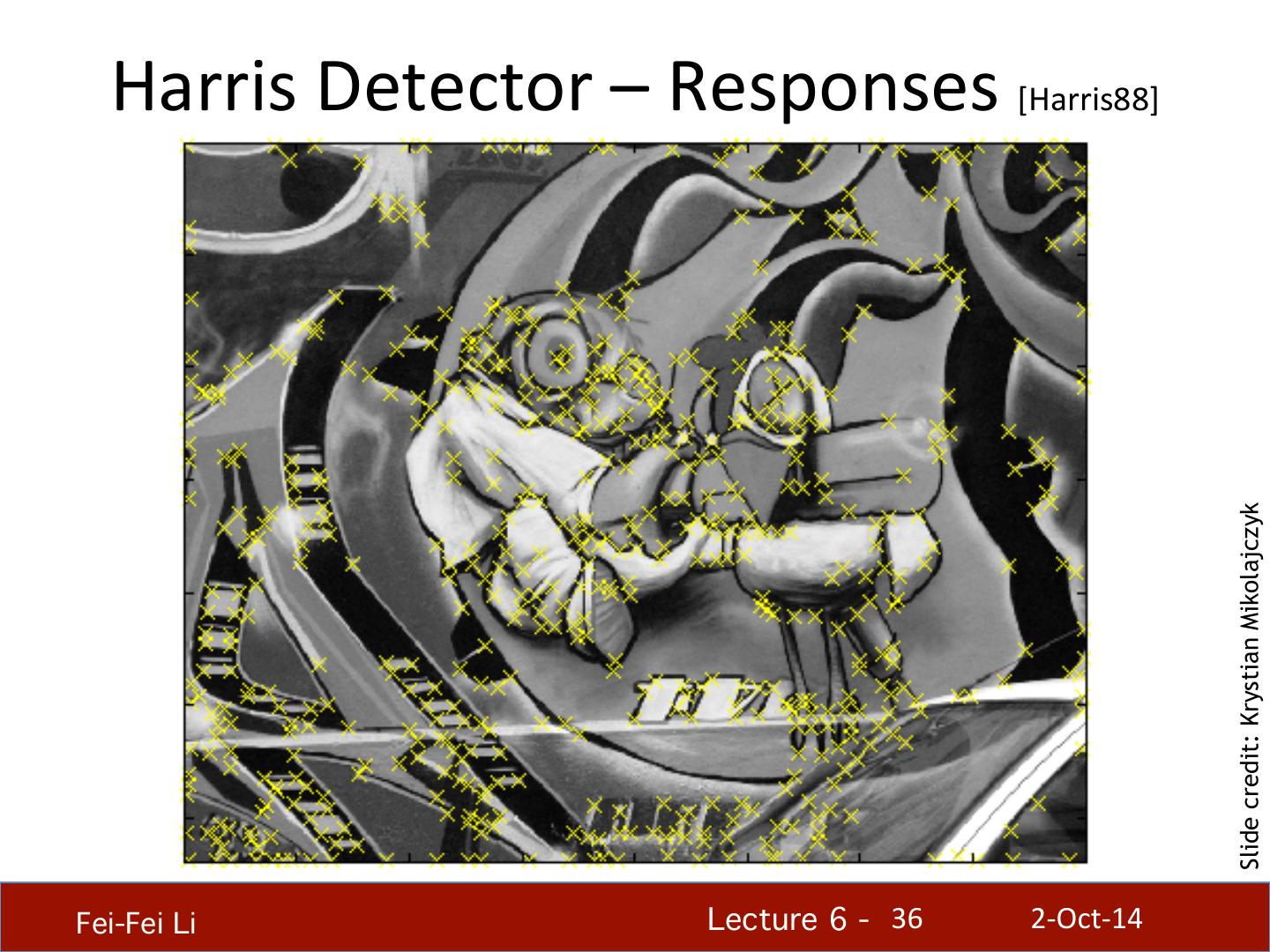
19 . Finding Corners •  Key property: Slide credit: Svetlana Lazebnik –  In the region around a corner, image gradient has two or more dominant direcHons •  Corners are repeatable and dis8nc8ve C.Harris and M.Stephens. "A Combined Corner and Edge Detector.“ Proceedings of the 4th Alvey Vision Conference, 1988. Fei-Fei Li! Lecture 6 - !19 2-‐Oct-‐14

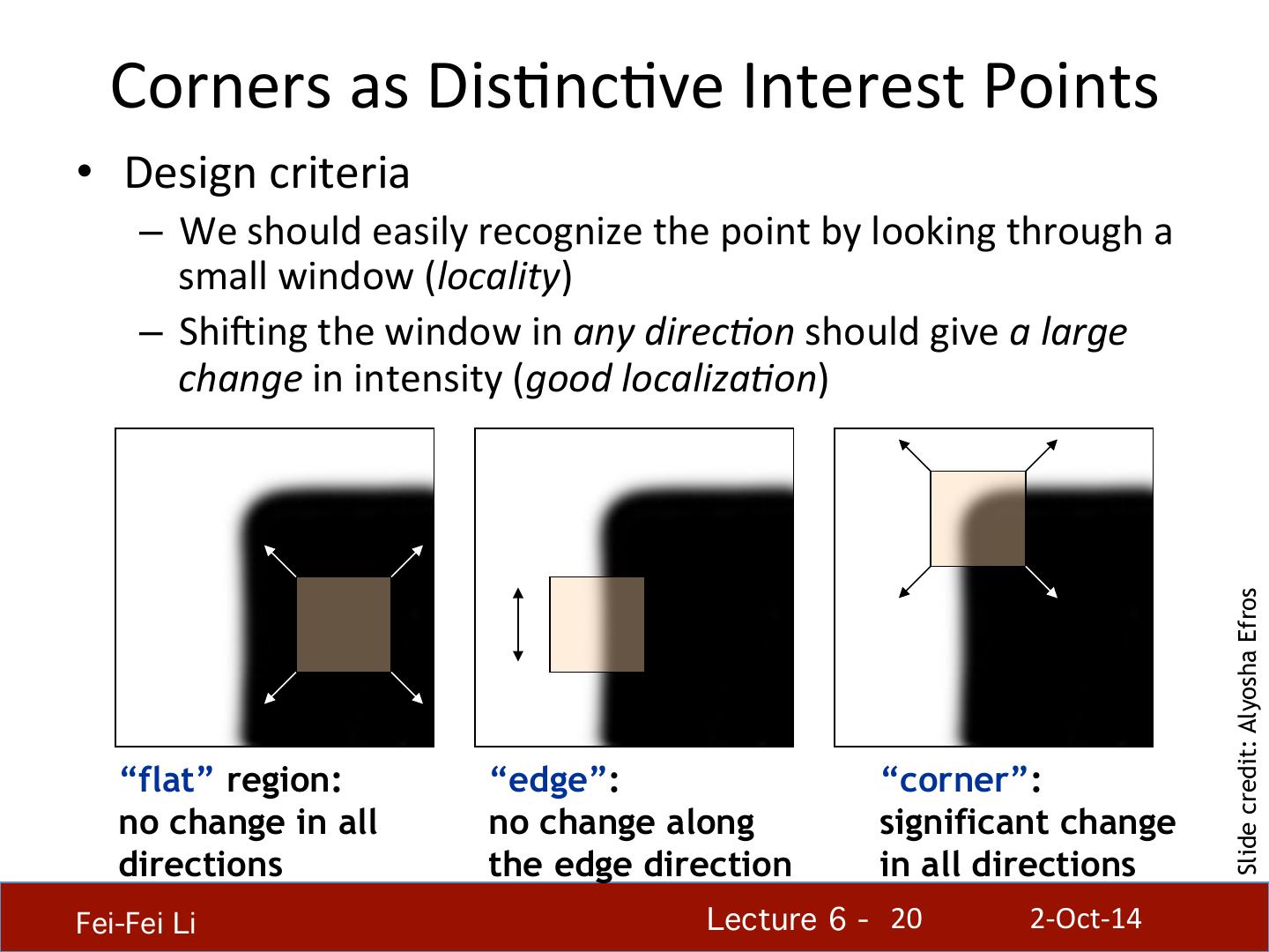
20 . Corners as DisHncHve Interest Points •  Design criteria –  We should easily recognize the point by looking through a small window (locality) –  Shifing the window in any direc8on should give a large change in intensity (good localiza8on) Slide credit: Alyosha Efros “flat” region: “edge”: “corner”: no change in all no change along significant change directions the edge direction in all directions Fei-Fei Li! Lecture 6 - !20 2-‐Oct-‐14

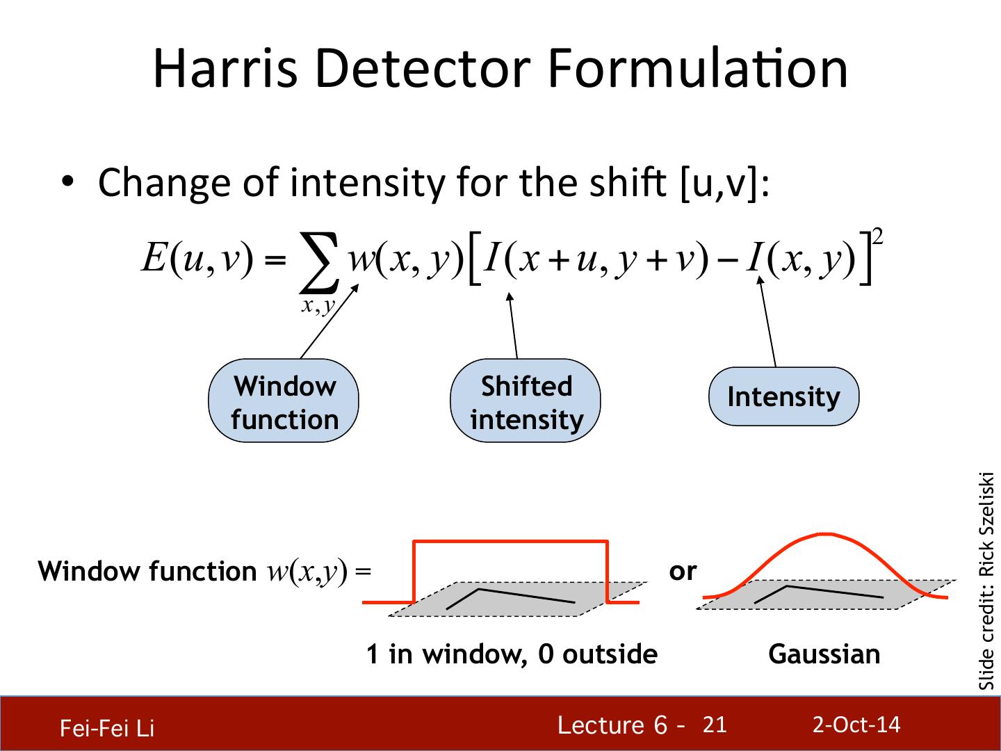
21 . Harris Detector FormulaHon •  Change of intensity for the shif [u,v]: 2 E (u, v) = ∑ w( x, y) [ I ( x + u, y + v) − I ( x, y) ] x, y Window Shifted Intensity function intensity Slide credit: Rick Szeliski Window function w(x,y) = or 1 in window, 0 outside Gaussian Fei-Fei Li! Lecture 6 - !21 2-‐Oct-‐14

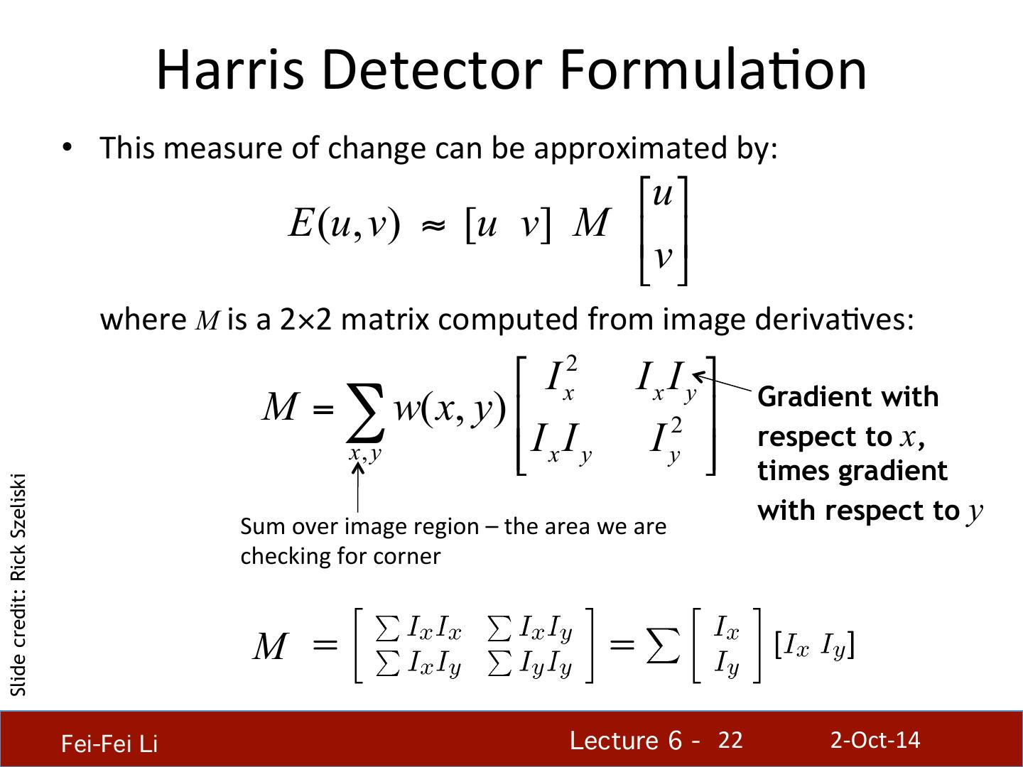
22 . Harris Detector FormulaHon •  This measure of change can be approximated by: ⎡u ⎤ E (u, v) ≈ [u v] M ⎢ ⎥ ⎣ v ⎦ where M is a 2×2 matrix computed from image derivaHves: ⎡ I x2 I x I y ⎤ Gradient with M = ∑ w( x, y) ⎢ 2 ⎥ x, y ⎢⎣ I x I y I y ⎥⎦ respect to x, times gradient Slide credit: Rick Szeliski with respect to y Sum over image region – the area we are checking for corner M Fei-Fei Li! Lecture 6 - !22 2-‐Oct-‐14

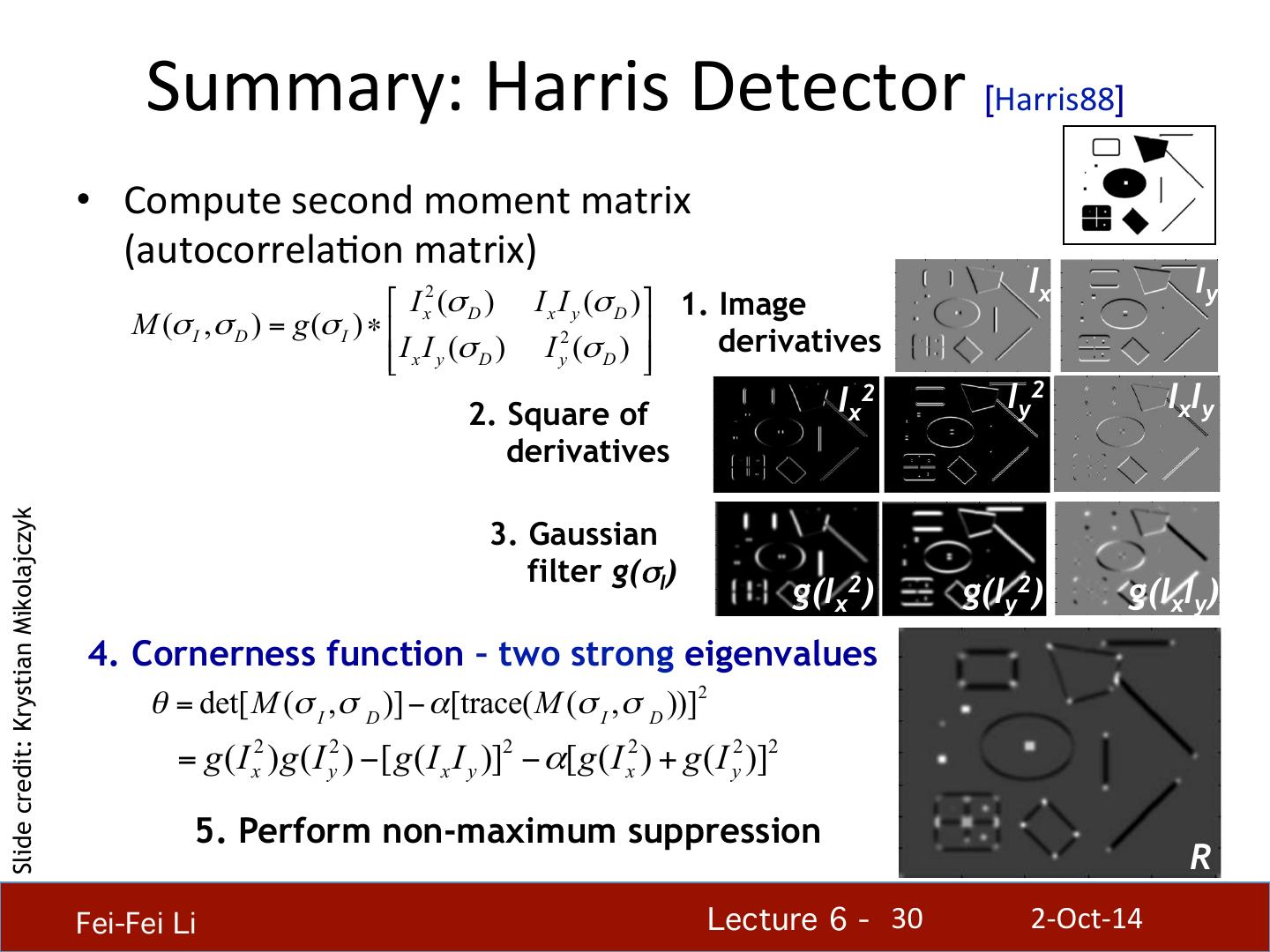
23 . Harris Detector FormulaHon Image I Ix Iy IxIy where M is a 2×2 matrix computed from image derivaHves: ⎡ I x2 I x I y ⎤ Gradient with M = ∑ w( x, y) ⎢ 2 ⎥ x, y ⎢⎣ I x I y I y ⎥⎦ respect to x, times gradient Slide credit: Rick Szeliski with respect to y Sum over image region – the area we are checking for corner M Fei-Fei Li! Lecture 6 - !23 2-‐Oct-‐14

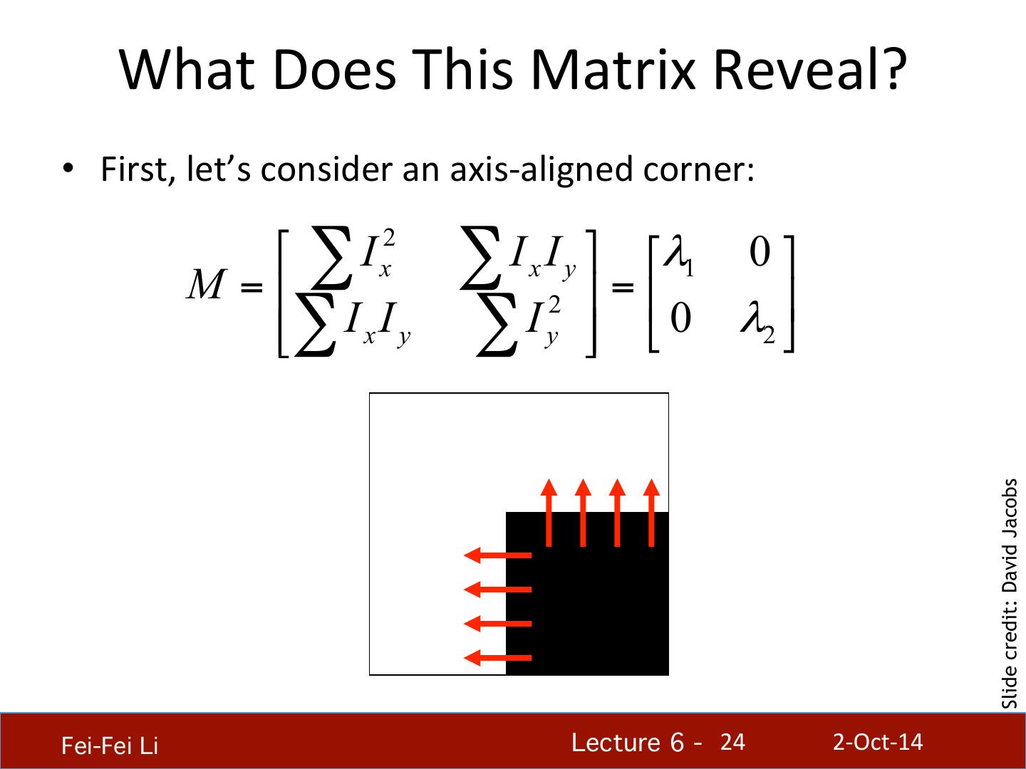
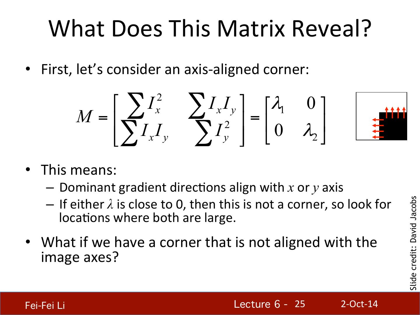
24 . What Does This Matrix Reveal? •  First, let’s consider an axis-‐aligned corner: ⎡ ∑ I x2 ∑I I x y ⎤ ⎡λ1 0 ⎤ M = ⎢ 2 ⎥ = ⎢ ⎥ ⎢⎣∑ I x I y ∑I y ⎥⎦ ⎣ 0 λ2 ⎦ •  This means: –  Dominant gradient direcHons align with x or y axis –  If either λ is close to 0, then this is not a corner, so look for Slide credit: David Jacobs locaHons where both are large. •  What if we have a corner that is not aligned with the image axes? Fei-Fei Li! Lecture 6 - !24 2-‐Oct-‐14

25 . What Does This Matrix Reveal? •  First, let’s consider an axis-‐aligned corner: ⎡ ∑ I x2 ∑I I x y ⎤ ⎡λ1 0 ⎤ M = ⎢ 2 ⎥ = ⎢ ⎥ ⎢⎣∑ I x I y ∑I y ⎥⎦ ⎣ 0 λ2 ⎦ •  This means: –  Dominant gradient direcHons align with x or y axis –  If either λ is close to 0, then this is not a corner, so look for Slide credit: David Jacobs locaHons where both are large. •  What if we have a corner that is not aligned with the image axes? Fei-Fei Li! Lecture 6 - !25 2-‐Oct-‐14

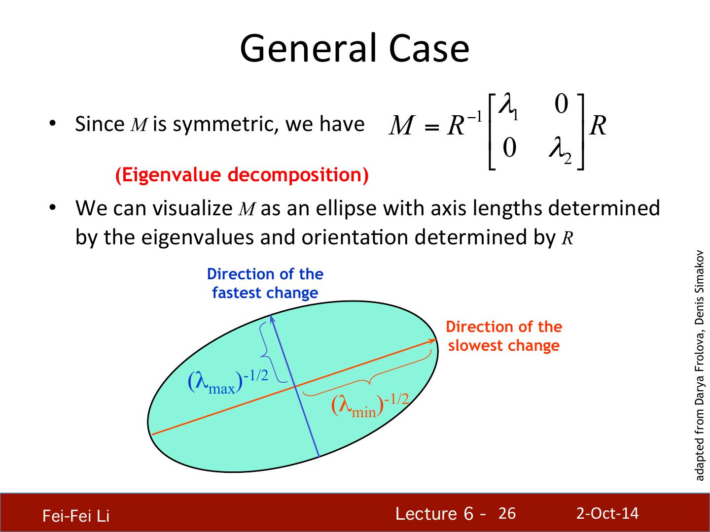
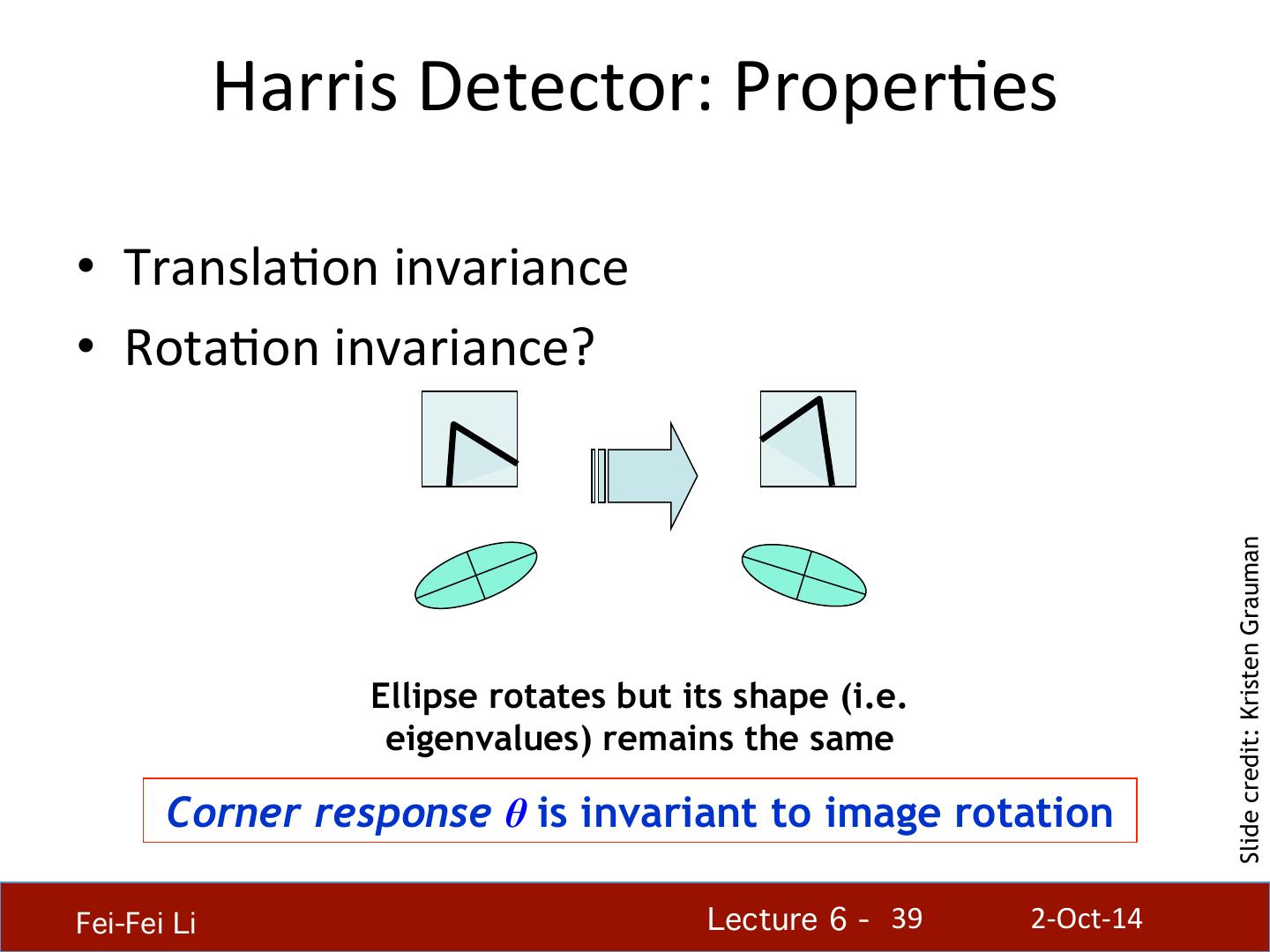
26 . General Case ⎡λ1 0 ⎤ −1 •  Since M is symmetric, we have M = R ⎢ 0 λ ⎥ R ⎣ 2 ⎦ (Eigenvalue decomposition) •  We can visualize M as an ellipse with axis lengths determined by the eigenvalues and orientaHon determined by R adapted from Darya Frolova, Denis Simakov Direction of the fastest change Direction of the slowest change (λmax)-1/2 (λmin)-1/2 Fei-Fei Li! Lecture 6 - !26 2-‐Oct-‐14

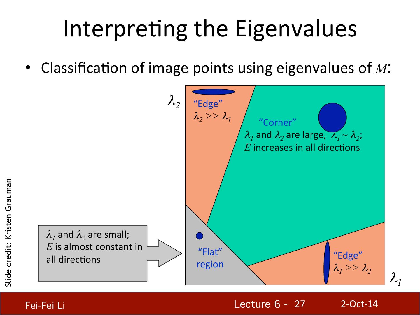
27 . InterpreHng the Eigenvalues •  ClassiﬁcaHon of image points using eigenvalues of M: λ2 “Edge” λ2 >> λ1 “Corner” λ1 and λ2 are large, λ1 ~ λ2; E increases in all direcHons Slide credit: Kristen Grauman λ1 and λ2 are small; E is almost constant in “Flat” “Edge” all direcHons region λ1 >> λ2 λ1 Fei-Fei Li! Lecture 6 - !27 2-‐Oct-‐14

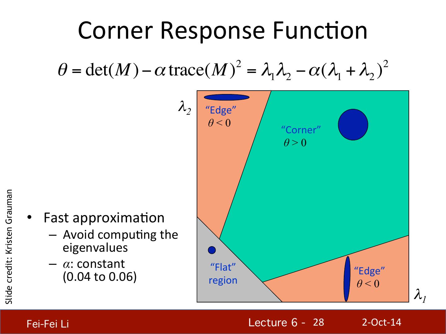
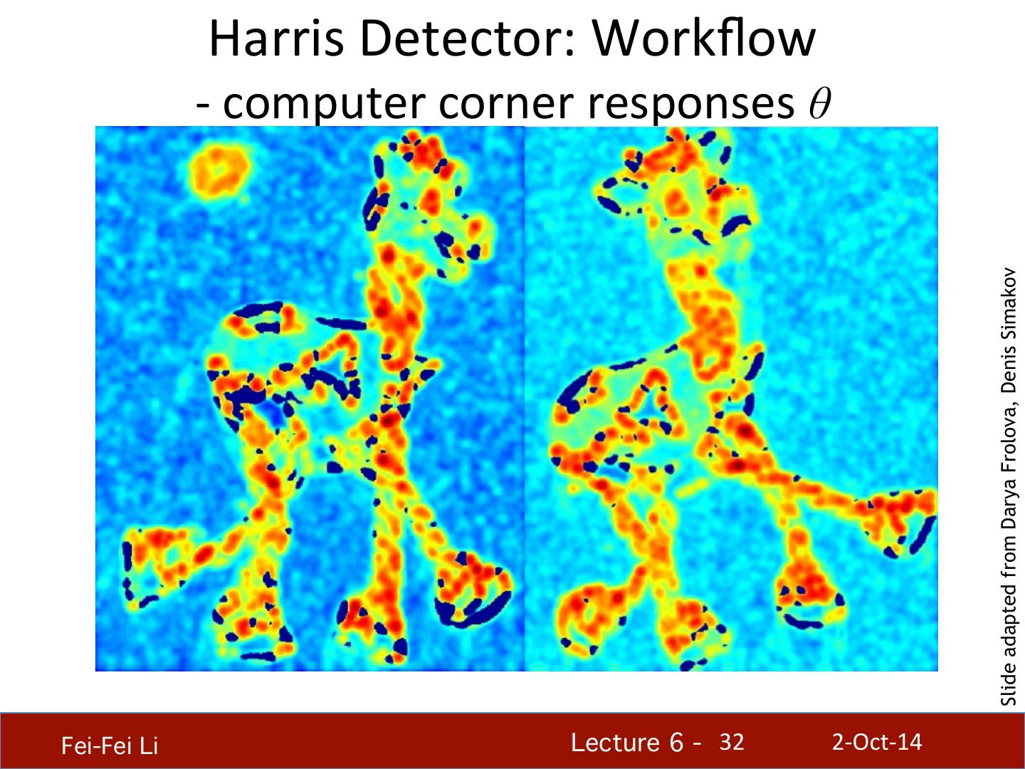
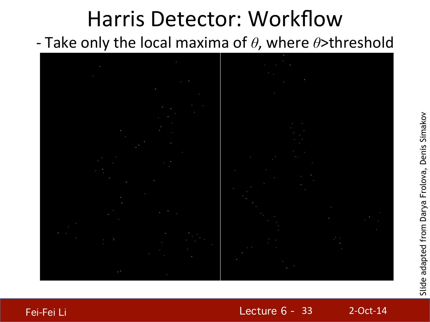
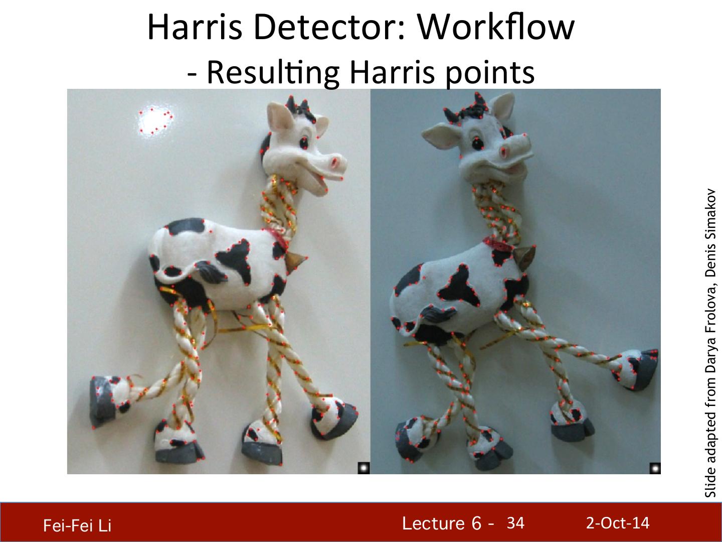
28 . Corner Response FuncHon θ = det(M ) − α trace(M )2 = λ1λ2 − α (λ1 + λ2 )2 λ2 “Edge” θ<0 “Corner” θ > 0 Slide credit: Kristen Grauman •  Fast approximaHon –  Avoid compuHng the eigenvalues –  α: constant “Flat” “Edge” (0.04 to 0.06) region θ<0 λ1 Fei-Fei Li! Lecture 6 - !28 2-‐Oct-‐14

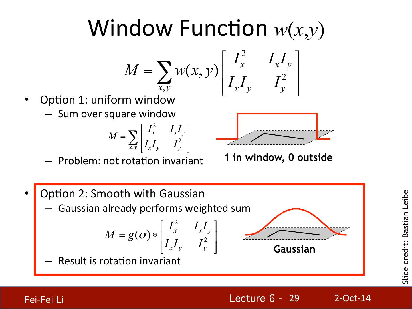
29 . Window FuncHon w(x,y) ⎡ I x2 I x I y ⎤ M = ∑ w( x, y) ⎢ 2 ⎥ x, y ⎢⎣ I x I y I y ⎥⎦ •  OpHon 1: uniform window –  Sum over square window ⎡ I x2 I x I y ⎤ M = ∑ ⎢ ⎥ ⎣ I x I y x , y ⎢ I y2 ⎥⎦ –  Problem: not rotaHon invariant 1 in window, 0 outside •  OpHon 2: Smooth with Gaussian Slide credit: Bastian Leibe –  Gaussian already performs weighted sum ⎡ I x2 I x I y ⎤ M = g (σ ) ∗ ⎢ 2 ⎥ I I ⎣⎢ x y I y ⎥⎦ Gaussian –  Result is rotaHon invariant Fei-Fei Li! Lecture 6 - !29 2-‐Oct-‐14

3点赞

2收藏

0下载