K-means Clustering

下载 0

乐乐

发布于

3117

人观看

#信息技术

k平均聚类发明于1956年，是一个聚类算法，把n的对象根据他们的属性分为k个分割，k < n。它与处理混合正态分布的最大期望算法很相似，因为他们都试图找到数据中自然聚类的中心。它假设对象属性来自于空间向量，并且目标是使各个群组内部的均方误差总和最小。假设有k个群组Si, i=1,2,...,k。

展开查看详情

1 . Lecture 13: k-‐means and mean-‐shi4 clustering Professor Fei-‐Fei Li Stanford Vision Lab Fei-Fei Li! Lecture 13 - 1 ! 3-‐Nov-‐14

2 . Recap: Gestalt Theory •  Gestalt: whole or group –  Whole is greater than sum of its parts –  RelaHonships among parts can yield new properHes/features •  Psychologists idenHﬁed series of factors that predispose set of elements to be grouped (by human visual system) “I stand at the window and see a house, trees, sky. Theoretically I might say there were 327 brightnesses and nuances of colour. Do I have "327"? No. I have sky, house, and trees.” Max Wertheimer (1880-1943) Untersuchungen zur Lehre von der Gestalt, Psychologische Forschung, Vol. 4, pp. 301-350, 1923 http://psy.ed.asu.edu/~classics/Wertheimer/Forms/forms.htm Fei-Fei Li! Lecture 13 - 2 ! 3-‐Nov-‐14

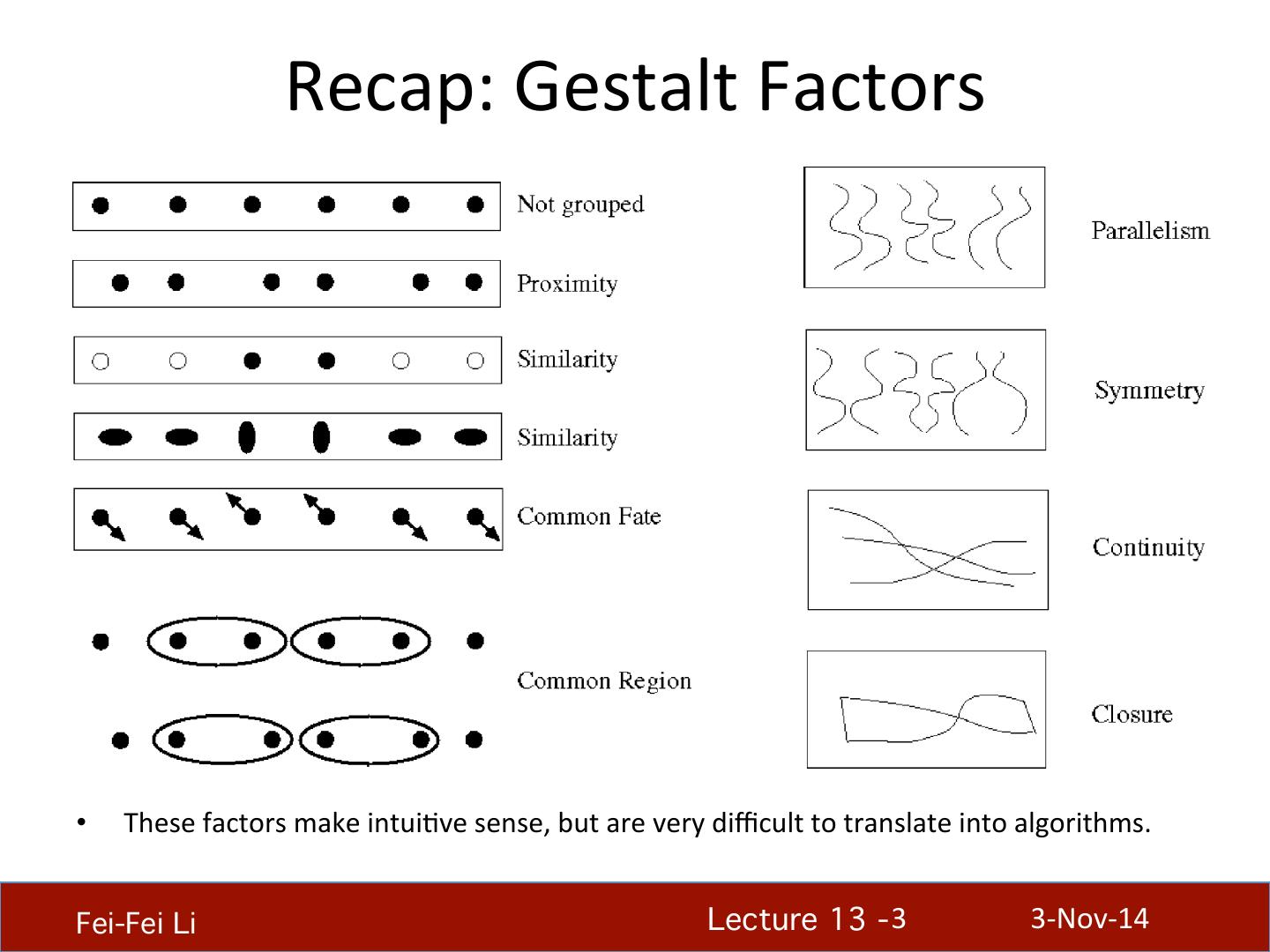
3 . Recap: Gestalt Factors •  These factors make intuiHve sense, but are very diﬃcult to translate into algorithms. Fei-Fei Li! Lecture 13 - 3 ! 3-‐Nov-‐14

4 . Recap: Image SegmentaHon •  Goal: idenHfy groups of pixels that go together Fei-Fei Li! Lecture 13 - 4 ! 3-‐Nov-‐14

5 . What will we learn today? •  K-‐means clustering •  Mean-‐shi4 clustering Reading: [FP] Chapters: 14.2, 14.4 D. Comaniciu and P. Meer, Mean Shi4: A Robust Approach toward Feature Space Analysis, PAMI 2002. Fei-Fei Li! Lecture 13 - 5 ! 3-‐Nov-‐14

6 . What will we learn today? •  K-‐means clustering •  Mean-‐shi4 clustering Reading: [FP] Chapters: 14.2, 14.4 D. Comaniciu and P. Meer, Mean Shi4: A Robust Approach toward Feature Space Analysis, PAMI 2002. Fei-Fei Li! Lecture 13 - 6 ! 3-‐Nov-‐14

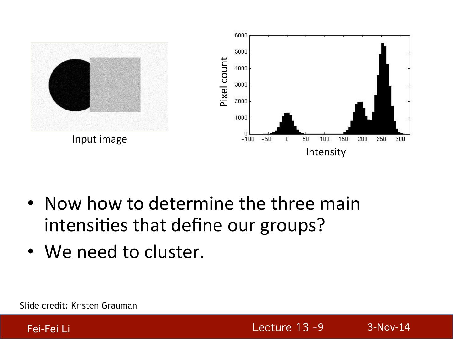
7 . Image SegmentaHon: Toy Example white pixels 3 black pixels gray 1 2 pixels input image intensity •  These intensiHes deﬁne the three groups. •  We could label every pixel in the image according to which of these primary intensiHes it is. –  i.e., segment the image based on the intensity feature. •  What if the image isn’t quite so simple? Slide credit: Kristen Grauman Fei-Fei Li! Lecture 13 - 7 ! 3-‐Nov-‐14

8 . Pixel count Input image Intensity Pixel count Input image Intensity Slide credit: Kristen Grauman Fei-Fei Li! Lecture 13 - 8 ! 3-‐Nov-‐14

9 . Pixel count Input image Intensity •  Now how to determine the three main intensiHes that deﬁne our groups? •  We need to cluster. Slide credit: Kristen Grauman Fei-Fei Li! Lecture 13 - 9 ! 3-‐Nov-‐14

10 . 0 190 255 Intensity 3 1 2 •  Goal: choose three “centers” as the representaHve intensiHes, and label every pixel according to which of these centers it is nearest to. Slide credit: Kristen Grauman •  Best cluster centers are those that minimize Sum of Square Distance (SSD) between all points and their nearest cluster center ci: 2 SSD = ∑ ∑ ( x − ci ) clusteri x∈clusteri Fei-Fei Li! Lecture 13 - 10 ! 3-‐Nov-‐14

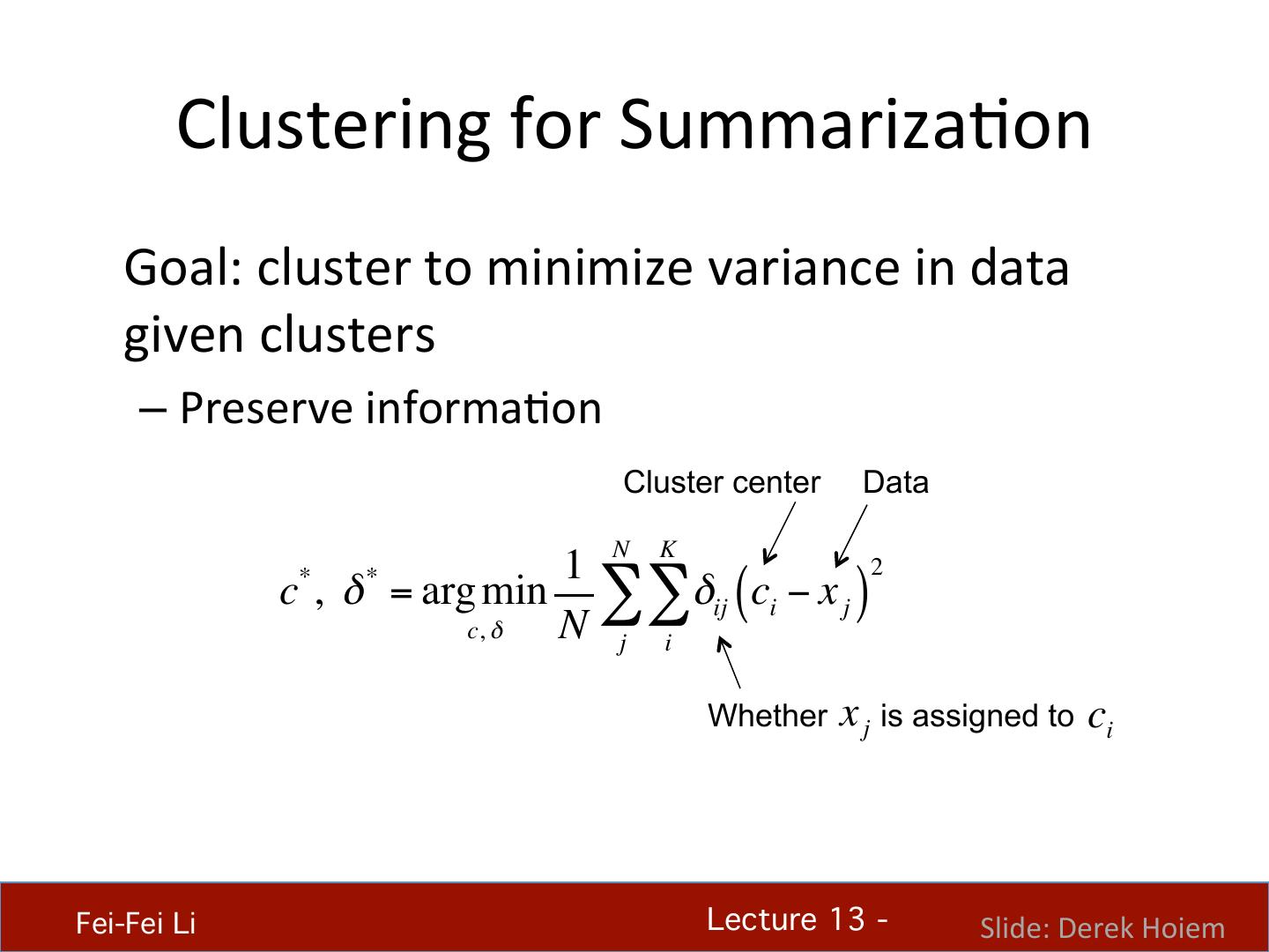
11 . Clustering for SummarizaHon Goal: cluster to minimize variance in data given clusters –  Preserve informaHon Cluster center Data 1 N K 2 c , δ = arg min ∑∑δij ( ci − x j ) * * c, δ N j i Whether x j is assigned to ci Fei-Fei Li! Lecture 13 - ! Slide: Derek Hoiem

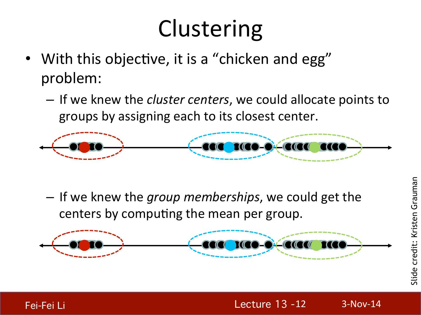
12 . Clustering •  With this objecHve, it is a “chicken and egg” problem: –  If we knew the cluster centers, we could allocate points to groups by assigning each to its closest center. Slide credit: Kristen Grauman –  If we knew the group memberships, we could get the centers by compuHng the mean per group. Fei-Fei Li! Lecture 13 - 12 ! 3-‐Nov-‐14

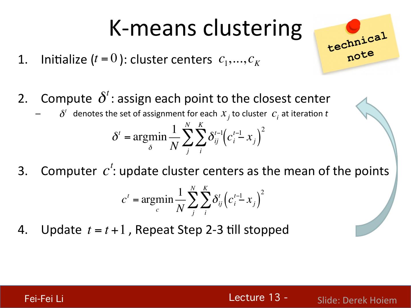
13 . K-‐means clustering h n i cal tec 1.  IniHalize (t = 0 ): cluster centers c1,..., cK note t 2.  Compute δ : assign each point to the closest center –  δ t denotes the set of assignment for each x j to cluster c i at iteraHon t N K 1 2 δ = argmin ∑∑δ ij ( ci − x j ) t t−1 t−1 δ N j i t 3.  Computer c : update cluster centers as the mean of the points 1 N K t t−1 2 t c = argmin ∑ ∑ δ (c − x ) ij i j c N j i 4.  Update t = t +1 , Repeat Step 2-‐3 Hll stopped Fei-Fei Li! Lecture 13 - ! Slide: Derek Hoiem

14 . K-‐means clustering h n i cal tec 1.  IniHalize (t = 0 ): cluster centers c1,..., cK note •  Commonly used: random iniHalizaHon •  Or greedily choose K to minimize residual t 2.  Compute δ : assign each point to the closest center •  Typical distance measure: •  Euclidean sim(x, x!) = x T x! •  Cosine sim(x, x!) = x T x! (x ⋅ x! ) •  Others t 3.  Computer c : update cluster centers as the mean of the points 1 N K t t−1 2 c = argmin ∑∑δ ij ( ci − x j ) t c N j i 4.  Update t = t +1 , Repeat Step 2-‐3 Hll stopped t •  c doesn’t change anymore. Fei-Fei Li! Lecture 13 - ! Slide: Derek Hoiem

15 . K-‐means clustering 1. Initialize 2. Assign Points to 3. Re-compute Repeat (2) and (3) Cluster Centers Clusters Means •  Java demo: hmp://home.dei.polimi.it/mameucc/Clustering/tutorial_html/AppletKM.html Fei-Fei Li! Lecture 13 - ! Illustration Source: wikipedia

16 . K-‐means clustering h n i cal tec note •  Converges to a local minimum soluHon –  IniHalize mulHple runs •  Bemer ﬁt for spherical data •  Need to pick K (# of clusters) Fei-Fei Li! Lecture 13 - 16 ! 3-‐Nov-‐14

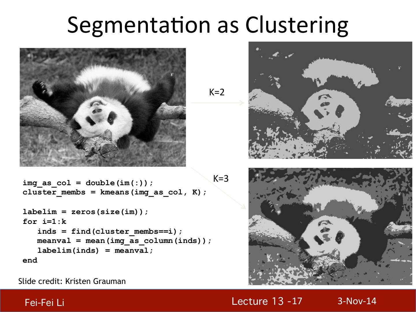
17 . SegmentaHon as Clustering K=2 img_as_col = double(im(:)); K=3 cluster_membs = kmeans(img_as_col, K); labelim = zeros(size(im)); for i=1:k inds = find(cluster_membs==i); meanval = mean(img_as_column(inds)); labelim(inds) = meanval; end Slide credit: Kristen Grauman Fei-Fei Li! Lecture 13 - 17 ! 3-‐Nov-‐14

18 . K-‐Means++ •  Can we prevent arbitrarily bad local minima? 1. Randomly choose ﬁrst center. 2 2. Pick new center with prob. proporHonal to ( x − ci) –  (ContribuHon of x to total error) 3. Repeat unHl K centers. Slide credit: Steve Seitz •  Expected error = O ( log K ) * opHmal Arthur & Vassilvitskii 2007 Fei-Fei Li! Lecture 13 - 18 ! 3-‐Nov-‐14

19 . Feature Space •  Depending on what we choose as the feature space, we can group pixels in diﬀerent ways. •  Grouping pixels based on intensity similarity •  Feature space: intensity value (1D) Slide credit: Kristen Grauman Fei-Fei Li! Lecture 13 - 19 ! 3-‐Nov-‐14

20 . Feature Space •  Depending on what we choose as the feature space, we can group pixels in diﬀerent ways. R=255 G=200 •  Grouping pixels based B=250 on color similarity B R=245 G G=220 B=248 R R=15 R=3 G=189 G=12 B=2 B=2 •  Feature space: color value (3D) Slide credit: Kristen Grauman Fei-Fei Li! Lecture 13 - 20 ! 3-‐Nov-‐14

21 . Feature Space •  Depending on what we choose as the feature space, we can group pixels in diﬀerent ways. •  Grouping pixels based on texture similarity F1 F2 Filter bank of 24 ﬁlters … F24 •  Feature space: ﬁlter bank responses (e.g., 24D) Slide credit: Kristen Grauman Fei-Fei Li! Lecture 13 - 21 ! 3-‐Nov-‐14

22 . Smoothing Out Cluster Assignments •  Assigning a cluster label per pixel may yield outliers: Original Labeled by cluster center’s intensity ? •  How can we ensure they 3 are spaHally smooth? 1 2 Slide credit: Kristen Grauman Fei-Fei Li! Lecture 13 - 22 ! 3-‐Nov-‐14

23 . SegmentaHon as Clustering •  Depending on what we choose as the feature space, we can group pixels in diﬀerent ways. •  Grouping pixels based on intensity+posi9on similarity Intensity Y X ⇒ Way to encode both similarity and proximity. Slide credit: Kristen Grauman Fei-Fei Li! Lecture 13 - 23 ! 3-‐Nov-‐14

24 . K-‐Means Clustering Results •  K-‐means clustering based on intensity or color is essenHally vector quanHzaHon of the image amributes –  Clusters don’t have to be spaHally coherent Image Intensity-‐based clusters Color-‐based clusters Image source: Forsyth & Ponce Fei-Fei Li! Lecture 13 - 24 ! 3-‐Nov-‐14

25 . K-‐Means Clustering Results •  K-‐means clustering based on intensity or color is essenHally vector quanHzaHon of the image amributes –  Clusters don’t have to be spaHally coherent •  Clustering based on (r,g,b,x,y) values enforces more spaHal coherence Image source: Forsyth & Ponce Fei-Fei Li! Lecture 13 - 25 ! 3-‐Nov-‐14

26 . How to evaluate clusters? •  GeneraHve –  How well are points reconstructed from the clusters? •  DiscriminaHve –  How well do the clusters correspond to labels? •  Purity –  Note: unsupervised clustering does not aim to be discriminaHve Fei-Fei Li! Lecture 13 - ! Slide: Derek Hoiem

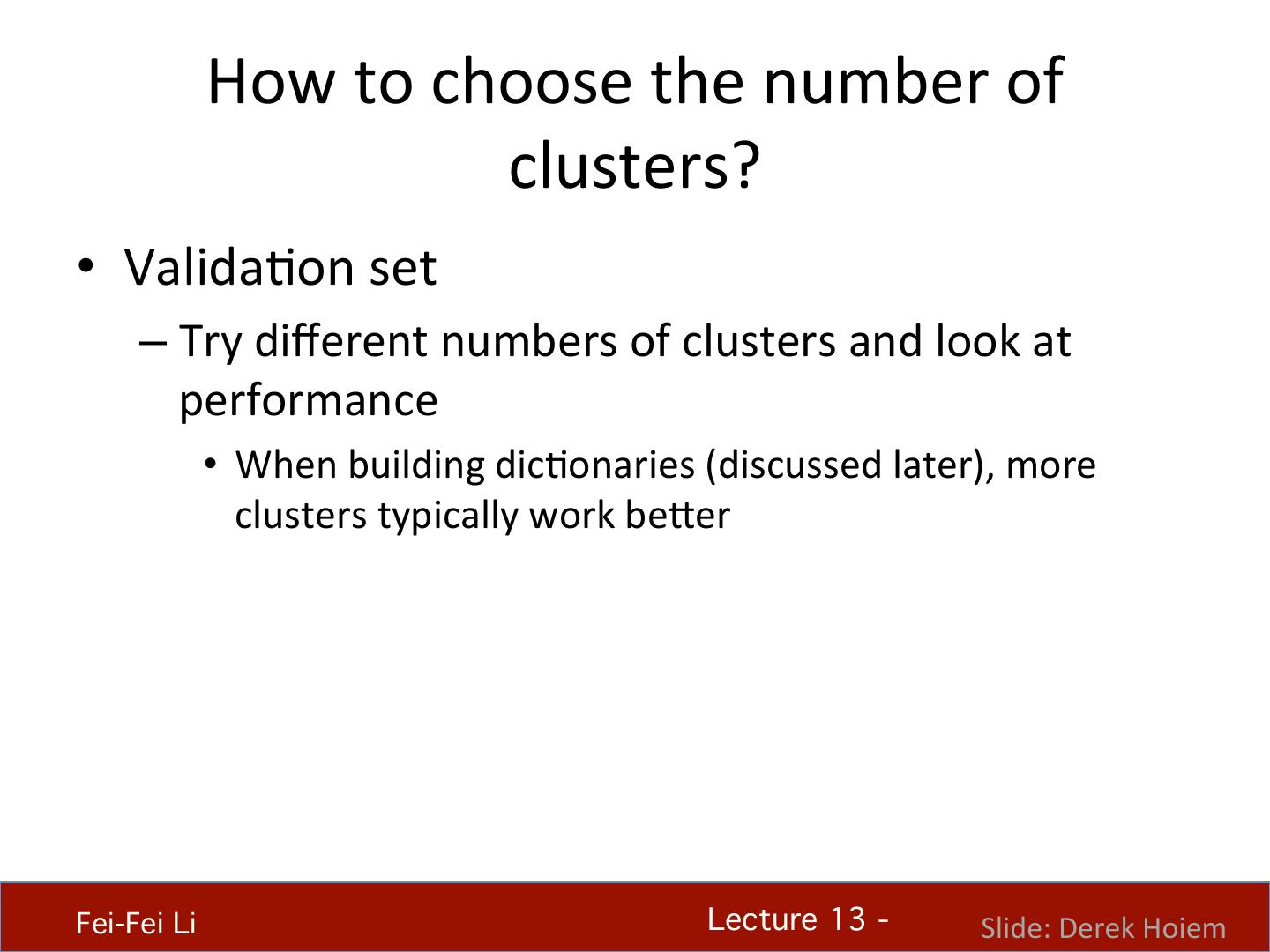
27 . How to choose the number of clusters? •  ValidaHon set –  Try diﬀerent numbers of clusters and look at performance •  When building dicHonaries (discussed later), more clusters typically work bemer Fei-Fei Li! Lecture 13 - ! Slide: Derek Hoiem

28 . K-‐Means pros and cons •  Pros •  Finds cluster centers that minimize condiHonal variance (good representaHon of data) •  Simple and fast, Easy to implement •  Cons •  Need to choose K •  SensiHve to outliers •  Prone to local minima •  All clusters have the same parameters (e.g., distance measure is non-‐ adapHve) •  *Can be slow: each iteraHon is O(KNd) for N d-‐dimensional points •  Usage •  Unsupervised clustering •  Rarely used for pixel segmentaHon Fei-Fei Li! Lecture 13 - !

29 . What will we learn today? •  K-‐means clustering •  Mean-‐shi4 clustering Reading: [FP] Chapters: 14.2, 14.4 D. Comaniciu and P. Meer, Mean Shi4: A Robust Approach toward Feature Space Analysis, PAMI 2002. Fei-Fei Li! Lecture 13 - 29 ! 3-‐Nov-‐14

3点赞

1收藏

0下载