近似算法--品质因数.性能比

1 . Approximation Algorithms Subhash Suri November 27, 2017 1 Figure of Merit: Performance Ratio • Suppose we are working on an optimization problem in which each potential solution has a positive cost, and we want to find one of near-optimal cost. When the objective is to minimize the cost, the near-optimal is always going to be more than the optimal. When the objective is to maximize profit, the near-optimal is less that the optimal. • The standard measure (figure of merit) in Theory of Algorithms to measure the quality of approximation is the ratio: cost(A) ρ(n) = max , cost(OP T ) where the max is over all input instances of size n, and the objective function is minimizing. If the objective is a maximization, then we choose profit(OP T ) ρ(n) = max profit(A) 2 Approximating the Vertex Cover • Given a graph G = (V, E), find a vertex cover C ⊆ V of minimize size; that is, for each edge (u, v) ∈ E, either u or v is in C. – cost(A) = size of VC found by our algorithm A; – cost(OP T ) = optimal VC size – ρ(n) = max (worst-case) value of cost(A)/cost(OP T ) over all n node graphs 1 

2 .• This problem seems well-suited for greedy strategies. Perhaps the most obvious and natural greedy scheme is the following: – repeatedly choose the vertex that covers most edges until no edges left uncovered. • The number of edges covered by a vertex v is its degree d(v). So, we repeatedly choose the max-deg vertex, delete all of its incident edges, and repeat, until no edges left. • An example graph. • When does it not find the optimal? How poorly can this algorithm perform in worst case? Is the worst-case ratio bounded (doesn’t grow with n)? • Unfortunately not! • Counter-example is bipartite graph: Gn = (L + R, E), where L is a set of n vertices 1, 2, . . . , n. • Then, for each i = 2, 3, . . . , n, we add another set of vertices Ri where |Ri | = n/i , and each vertex of Ri is then joined to i distinct vertices of L. Thus, each vertex of Ri has degree i. • Rn consists of 1 vertex, connected to everyone in L. Ri−1 also consists of a single vertex, connected to 1, 2, . . . , n − 1. R2 has n/2 vertices, each of degree 2. • If we run the greedy algorithm on this example, we will first choose Rn , then Rn−1 , and so on until we choose all the vertices of R. How many vertices are in R? n/2 + n/3 + n/4 + . . . 1 = Ω(n log n). • So, cost(A) = Θ(n log n). • However, OPT could have just chosen all the vertices of L, of which there are only n. • So, the ratio is at least Ω(log n)! • Now, instead consider another simple greedy scheme: – while E not empty, 1. pick an arbitrary edge e = (u, v) 2. add both u and v to C 3. delete all edges from E incident to u or v 2 

3 . • Example. • Theorem: The second greedy Vertex Cover algorithm has size at most twice the optimal. • Analysis. Let A be the set of edges picked by the greedy. Since no two edges in A can share a vertex, each of them requires a separate vertex in OPT to cover. So, OP T ≥ |A|. On the other hand, our greedy cover has size |C| ≤ 2|A|. QED. • Interestingly, the more natural greedy strategy of repeatedly picking the vertex of max degree can only achieve an approximation ratio log n. 3 Approximating the Traveling Salesman Tour • Input: G = (V, E), a complete graph, where each edge e has a positive cost w(e). • Output: The minimum cost tour visiting all the vertices of G exactly once. • General Impossibility Theorem. There is no polynomial-time algorithm to ap- proximate TSP to any factor unless N P = P . • Proof. – Suppose there is an algorithm that guarantees factor X approximation for TSP in polynomial time. We prove its impossibility by showing that such an algorithm can solve the HAMILTON cycle problem in polynomial time. – Given an instane G = (V, E) of the HAM problem, construct a TSP instance G as follows. – Set w(e) = 1 if e ∈ E, and w(e) = (nX + 1) if e ∈ E. – Now ask if G contains a TSP of cost ≤ n. – If G contains a HAM cycle, then the corresponding TSP has cost n, using the HAM cycle edges, each of cost one. – The approximation algorithm A must find a tour with cost ≤ nX. – Since each edge that is not in G has cost > nX, it cannot use that edge. So, the only tours that lead to acceptable approximation are the HAM cycles in G. – Conversely, if TSP returns a tour that costs more than nX, it must mean that G does not contain a HAM cycle. 3 

4 .3.1 TSP with Triangle Inequality • The good news about TSP is that if the edge costs satisfy triangle inequality, that is, w(a, b) ≤ w(a, c) + w(c, b), for any a, b, c, then we can approx the tour quite well. • Factor 2 approximation using MST. 4 Load balancing: minimizing MakeSpan • Problem: Given a set of m machines M1 , . . . , Mm , and a set of n jobs, where job j needs tj time for processing, the goal is to schedule the jobs on these machines so all the jobs are finished as soon as possible. • That is, find the minimum time (called MakeSpan) T by which all jobs can be executed collectively. • Let Ai be the set of jobs assigned to machine Mi . Then, Mi needs time Ti = tj j∈Ai this is called the load on machine Mi . We wish to minimize T = maxi {Ti }, which is called the makespan. • The decision problem is N P -complete: it’s in N P because we can decide whether the makespan is T or not. For completeness, we can reduce subset sum to it (scheduling on two machines). • We show that the following simple greedy method gives good approximation. The algorithm makes one pass over the jobs in any order, and assigns the next job j to the machine with the lightest current load. • for j = 1, . . . , n 1. Let Mi be the machine with the minimum Ti among the machines 2. Assign j to Mi 3. Ai = Ai ∪ {j} 4. Ti = Ti + tj 4 

5 .• For instance, given 6 jobs, with sizes 2, 3, 4, 6, 2, 3, and 3 machines, the algorithm gives (2, 6), (3, 2), (4, 3), for the makespan of 8. The optimal makespan is 7: (3, 4), (6), (2, 2, 3). • Analysis: Let T be the makespan produced by the algorithm, and T ∗ the optimal. • Note that, unfortunately, we do not know the value of T ∗ . Nevertheless, we can use a lower bound for T ∗ to achieve an approximation guaranteee. • A simple lower bound comes from the following trivial observation: since there is a total of j tj amount of work to be done by the m machines collectively, the makespan cannot be less than the avg load. Thus, 1 T∗ ≥ tj (1) m j • Unfortunately, this lower bound itself can be too weak: for instance, if we have one extremely long job, then the best we can do is to put it by itself on a single machine, but still the makespan has to be as long as this job. This greedy solution is optimal, but the lower bound may be way off, if the remaining jobs are all very small. But this suggests another lower bound: T ∗ ≥ maxj {tj } (2) • Theorem: The greedy makespan produces an assignment with makespan T ≤ 2T ∗ . • Proof. Look at the machine that attains the max load (makespan). Let this be Mi . • Let j be the last job assigned to Mi . • Key Observation: When j was assigned, Mi was the machine with the least load! Its load just before assignment of j was Ti − tj . • Since this was the lightest load, every other machine has load at least Ti − tj . Thus, adding up all these load, we have Tk ≥ m × (Ti − tj ) k equivalently, 1 Ti − tj ≤ Tk m k 5 

6 . • But the sum on the right is just the sum of all the jobs, since each job is assigned to some machine. The quantity on the RHS is just the lower bound from (1), and thus Ti − tj ≤ T ∗ • Now we account for the last job. Here we simply use the inequality (2), which says that tj <= T ∗ . Thus, Ti = (Ti − tj ) + tj ≤ 2T ∗ . QED. • It is easy to construct examples where this bound is tight. There is a better approx- imation: if we first sort the jobs in the decreasing order of lengths, and assign them using the greedy strategy, then one can show the approximation factor 3/2. 5 Set Cover • There is set U of n elements, and a list S1 , . . . , Sm of m subsets of U . A Set Cover is a collection of these sets whose union is U . Each set Si has a cost (or weight) wi , and our goal is to find a Set Cover of minimum weight. • Imagine U is a set of n baseball cards you wish to collect. The market offers bundles S1 , . . . , Sm that are subsets of U , at prices w1 , . . . , wm . You wish to collect all the cards in U at the minimum possible total cost. This is the set cover problem. • This is a fundamental NP-complete problem. We will develop a simple greedy algo- rithm for it, although the analysis is not trivial. • The first idea for the greedy is to repeatedly choose the largest set in the list. But this may not be good if the next set includes most of the items already covered (procured). So, a better idea may be to choose the next set that covers most items currently not covered! • Greedy-Set-Cover 1. Initialize R = U ; (set of remaining uncovered items) 2. while R not empty (a) Select set Si that minimizes |Siw∩R| i (b) Delete elements of Si from R 3. return selected sets • Picture 6 

7 .Analysis of the algorithm • The sets chosen by the algorithm clearly form a Set Cover. The main question is how much larger is the weight of this cover than the optimal w∗ . • Like the load balancing problem, we will need a lower bound for the optimal to compare, but unlike that problem, finding a good lower bound is more subtle and non-trivial. • Let us look at our greedy ”heuristic” and investigate the intuitive meaning of the ratio: wi /|Si ∩ R| • We can think of this as the cost paid for covering each new item. Suppose we “charge” this cost cs to each of the items s newly covered. Note that each item is charged a cost only once—when it is covered for the first time. • For bookkeeping only purpose, let’s add this line to the Greedy Algorithm when Si is added, to account for this cost. • First note that when Si is added, its weight is distributed even among the newly covered elements. Thus these costs simple account for the weights of the sets in the cover. • (Lemma 1:) If C is the greedy set cover, then wi = cs Si ∈C s∈U • The key to the proof is to ask: fix a particular set Sk . How much cost cs all the elements of Sk can incur? • In other words, compared to wk , how large is s∈Sk cs ? We derive an upper bound for any set Sk , even those not selected by the greedy. • (Lemma 2:) For any set Sk , cs ≤ wk × H(|Sk |), s∈Sk where H(n) = 1 + 1/2 + 1/3 + . . . + 1/n is the Harmonic number. • (Proof.) To simplify the notation, lets assume that the items of Sk are the first d = |Sk | items: s1 , s2 , . . . , sd . • Further, also assume that these items are labeled in the order in which they are assigned cost c by the greedy. (This is just renaming of items.) 7 

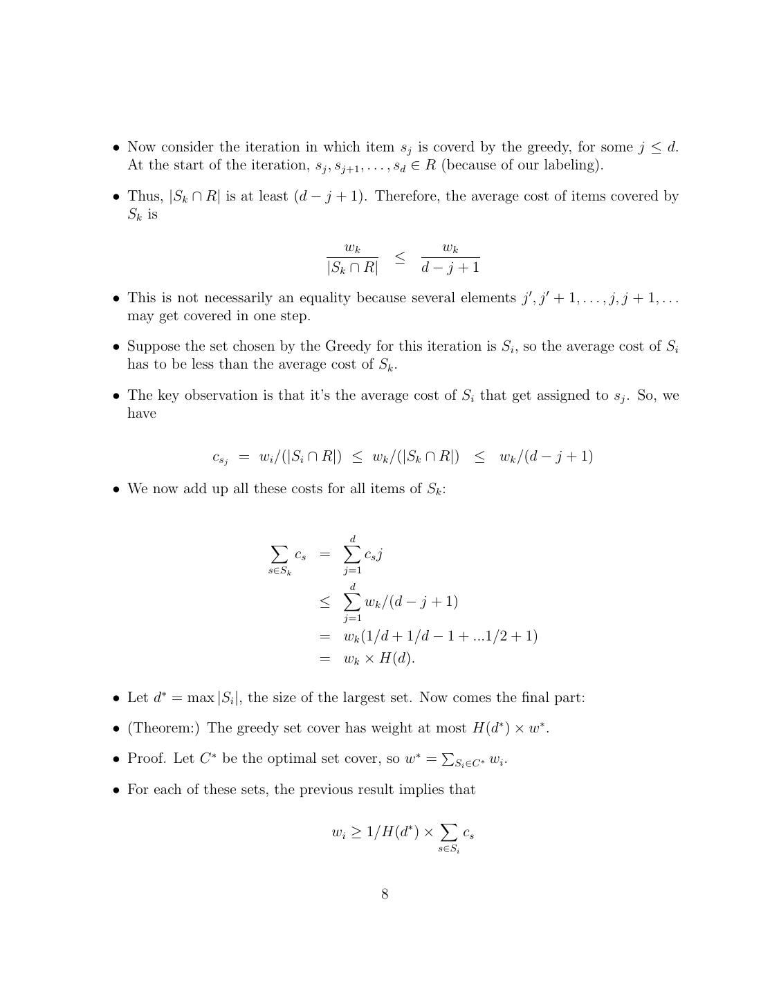
8 .• Now consider the iteration in which item sj is coverd by the greedy, for some j ≤ d. At the start of the iteration, sj , sj+1 , . . . , sd ∈ R (because of our labeling). • Thus, |Sk ∩ R| is at least (d − j + 1). Therefore, the average cost of items covered by Sk is wk wk ≤ |Sk ∩ R| d−j+1 • This is not necessarily an equality because several elements j , j + 1, . . . , j, j + 1, . . . may get covered in one step. • Suppose the set chosen by the Greedy for this iteration is Si , so the average cost of Si has to be less than the average cost of Sk . • The key observation is that it’s the average cost of Si that get assigned to sj . So, we have csj = wi /(|Si ∩ R|) ≤ wk /(|Sk ∩ R|) ≤ wk /(d − j + 1) • We now add up all these costs for all items of Sk : d cs = cs j s∈Sk j=1 d ≤ wk /(d − j + 1) j=1 = wk (1/d + 1/d − 1 + ...1/2 + 1) = wk × H(d). • Let d∗ = max |Si |, the size of the largest set. Now comes the final part: • (Theorem:) The greedy set cover has weight at most H(d∗ ) × w∗ . • Proof. Let C ∗ be the optimal set cover, so w∗ = Si ∈C ∗ wi . • For each of these sets, the previous result implies that wi ≥ 1/H(d∗ ) × cs s∈Si 8 

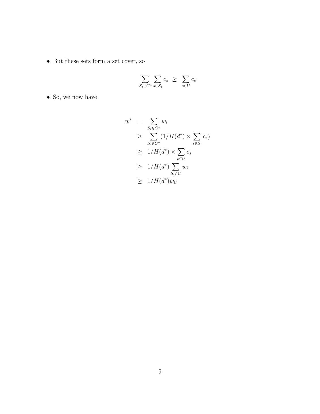
9 .• But these sets form a set cover, so cs ≥ cs Si ∈C ∗ s∈Si s∈U • So, we now have w∗ = wi Si ∈C ∗ ≥ (1/H(d∗ ) × cs ) Si ∈C ∗ s∈Si ≥ 1/H(d∗ ) × cs s∈U ≥ 1/H(d∗ ) wi Si ∈C ≥ 1/H(d∗ )wC 9