潜在语义索引

1 . More PCA; Latent Semantic Analysis and Multidimensional Scaling 36-350, Data Mining 21 September 2009 Reading: Principles of Data Mining, section 14.3.3 on latent semantic indexing. Contents 1 Latent Semantic Analysis: Yet More PCA and Yet More In- formation Retrieval 1 1.1 Principal Components of the Times Stories . . . . . . . . . . . . 3 2 PCA for Visualization 5 1 Latent Semantic Analysis: Yet More PCA and Yet More Information Retrieval Back when I was talking about abstraction, I mentioned that dimension reduc- tion is something that can be layered in between our original representations (like bags of words) and techniques that work in feature space (like similarity searching or nearest-neighbors). That is, rather than looking at the original features, we can apply the same procedures to the reduced, synthetic features we get from doing dimension reduction. This can have advantages in terms of speed (the vectors are smaller), memory (ditto) and even accuracy (since there are fewer parameters, explicit or implicit, to learn). One particularly nice application of this idea is to combine information re- trieval with the use of principal components in dimension reduction. This is called latent semantic analysis or latent semantic indexing. Remember from last time that the principal components we get from a collection of vec- tors depend on the covariance across the features. Features which are strongly correlated with each other will have projections on to the principal components which are very close to each other, while features which are weakly correlated or not at all will have nearly or exactly orthogonal projections — they’ll project on to different principal components. 1 

2 . Now suppose that the features are words in a big matrix of bag of word vectors. Two words being correlated means that they tend to appear together in the documents, or not at all. But this tendency needn’t be absolute — it can be partial because the words mean slightly different things, or because of stylistic differences, etc. But the projections of those features on to the principal components will generally be more similar than the original features are. To see how this can be useful, imagine we have a collection of documents (a corpus), which we want to search for documents about agriculture. It’s entirely possible that many documents on this topic don’t actually contain the word “agriculture”, just closely related words like “farming”. A simple feature-vector search on “agriculture” will miss them. But it’s very likely that the occurrence of these related words is well-correlated with the occurrence of “agriculture”. This means that all these words will have similar projections on to the principal components, so if we do similarity searching on the images of the query and the corpus, a search for “agriculture” will turn up documents that use “farming” a lot. To see why this is latent semantic indexing, think about what goes into coming up with an index for a book by hand. Someone draws up a list of topics and then goes through the book noting all the passages which refer to the topic, and maybe a little bit of what they say there. For example, here’s the start of the entry for “Agriculture” in the index to Adam Smith’s The Wealth of Nations: Agriculture, the labour of, does not admit of such subdivisions as manufactures, 6; this impossibility of separation, prevents agri- culture from improving equally with manufactures, 6; natural state of, in a new colony, 92; requires more knowledge and experience than most mechanical professions, and yet is carried on without any restrictions, 127; the terms of rent, how adjusted between landlord and tenant, 144; is extended by good roads and navigable canals, 147; under what circumstances pasture land is more valuable than arable, 149; gardening not a very gainful employment, 152–3; vines the most profitable article of culture, 154; estimates of profit from projects, very fallacious, ib.; cattle and tillage mutually improve each other, 220; . . . and so on. (Agriculture is an important topic in The Wealth of Nations.) It’s asking a lot to hope for a computer to be able to do something like this, but we could at least hope for a list of pages like “6, 92, 126, 144, 147, 152 − −3, 154, 220, . . .”. One could imagine doing this by treating each page as its own document, forming its bag-of-words vector, and then returning the list of pages with a non-zero entry for the feature “agriculture”. This will fail: only two of those nine pages actually contains that word, and this is pretty typical. On the other hand, they are full of words strongly correlated with “agriculture”, so asking for the pages which are most similar in their principal components 2 

3 .projection to that word will work great.1 At first glance, and maybe even second, this seems like a wonderful trick for extracting meaning (“semantics”) from pure correlations. Of course there are also all sorts of ways it can fail, not least from spurious correlations. If our training corpus happens to contain lots of documents which mention “farming” and “Kansas”, as well as “farming” and “agriculture”, latent semantic indexing will not make a big distinction between the relationship between “agriculture” and “farming” (which is genuinely semantic) and that between “Kansas” and “farming” (which is accidental, and probably wouldn’t show up in, say, a corpus collected from Europe). Despite this susceptibility to spurious correlations, latent semantic indexing is an extremely useful technique in practice, and the foundational papers (Deer- wester et al., 1990; Landauer and Dumais, 1997) are worth reading; you can find them on Blackboard or the course website. 1.1 Principal Components of the Times Stories To get a more concrete sense of how latent semantic analysis works, and how it reveals semantic information, let’s apply it to the Times stories. The ob- ject nyt.frame contains the stories, as usual, after inverse document frequency weighting and Euclidean length normalization, with the first column containing class labels. nyt.pca = prcomp(nyt.frame[,-1]) nyt.latent.sem = nyt.pca$rotation We need to omit the first column in the first command because it contains categorical variables, and PCA doesn’t apply to them. The second command just picks out the matrix of projections of the features on to the components — this is called rotation because it can be thought of as rotating the coordinate axes in feature-vector space. Now that we’ve done this, let’s look at what the leading components are. > signif(sort(nyt.latent.sem[,1],decreasing=TRUE)[1:30],2) music trio theater orchestra composers opera 0.110 0.084 0.083 0.067 0.059 0.058 theaters m festival east program y 0.055 0.054 0.051 0.049 0.048 0.048 jersey players committee sunday june concert 0.047 0.047 0.046 0.045 0.045 0.045 symphony organ matinee misstated instruments p 0.044 0.044 0.043 0.042 0.041 0.041 X.d april samuel jazz pianist society 0.041 0.040 0.040 0.039 0.038 0.038 > signif(sort(nyt.latent.sem[,1],decreasing=FALSE)[1:30],2) 1 Or it should anyway; I haven’t actually done the experiment with this book. 3 

4 . she her ms i said mother cooper -0.260 -0.240 -0.200 -0.150 -0.130 -0.110 -0.100 my painting process paintings im he mrs -0.094 -0.088 -0.071 -0.070 -0.068 -0.065 -0.065 me gagosian was picasso image sculpture baby -0.063 -0.062 -0.058 -0.057 -0.056 -0.056 -0.055 artists work photos you nature studio out -0.055 -0.054 -0.051 -0.051 -0.050 -0.050 -0.050 says like -0.050 -0.049 These are the thirty words with the largest positive and negative projections on to the first component.2 The words with positive projections are mostly associated with music, those with negative components with the visual arts. The letters “m” and “p” show up with msuic because of the combination “p.m”, which our parsing breaks into two single-letter words, and because stories about music give show-times more often than do stories about art. Personal pronouns appear with art stories because more of those quote people, such as artists or collectors.3 What about the second component? > signif(sort(nyt.latent.sem[,2],decreasing=TRUE)[1:30],2) art museum images artists donations museums 0.150 0.120 0.095 0.092 0.075 0.073 painting tax paintings sculpture gallery sculptures 0.073 0.070 0.065 0.060 0.055 0.051 painted white patterns artist nature service 0.050 0.050 0.047 0.047 0.046 0.046 decorative feet digital statue color computer 0.043 0.043 0.043 0.042 0.042 0.041 paris war collections diamond stone dealers 0.041 0.041 0.041 0.041 0.041 0.040 > signif(sort(nyt.latent.sem[,2],decreasing=FALSE)[1:30],2) her she theater opera ms -0.220 -0.220 -0.160 -0.130 -0.130 i hour production sang festival -0.083 -0.081 -0.075 -0.075 -0.074 music musical songs vocal orchestra -0.070 -0.070 -0.068 -0.067 -0.067 la singing matinee performance band -0.065 -0.065 -0.061 -0.061 -0.060 awards composers says my im -0.058 -0.058 -0.058 -0.056 -0.056 2 Which direction is positive and which negative is of course arbitrary; basically it depends on internal choices in the algorithm. 3 You should check out these explanations for yourself. 4 

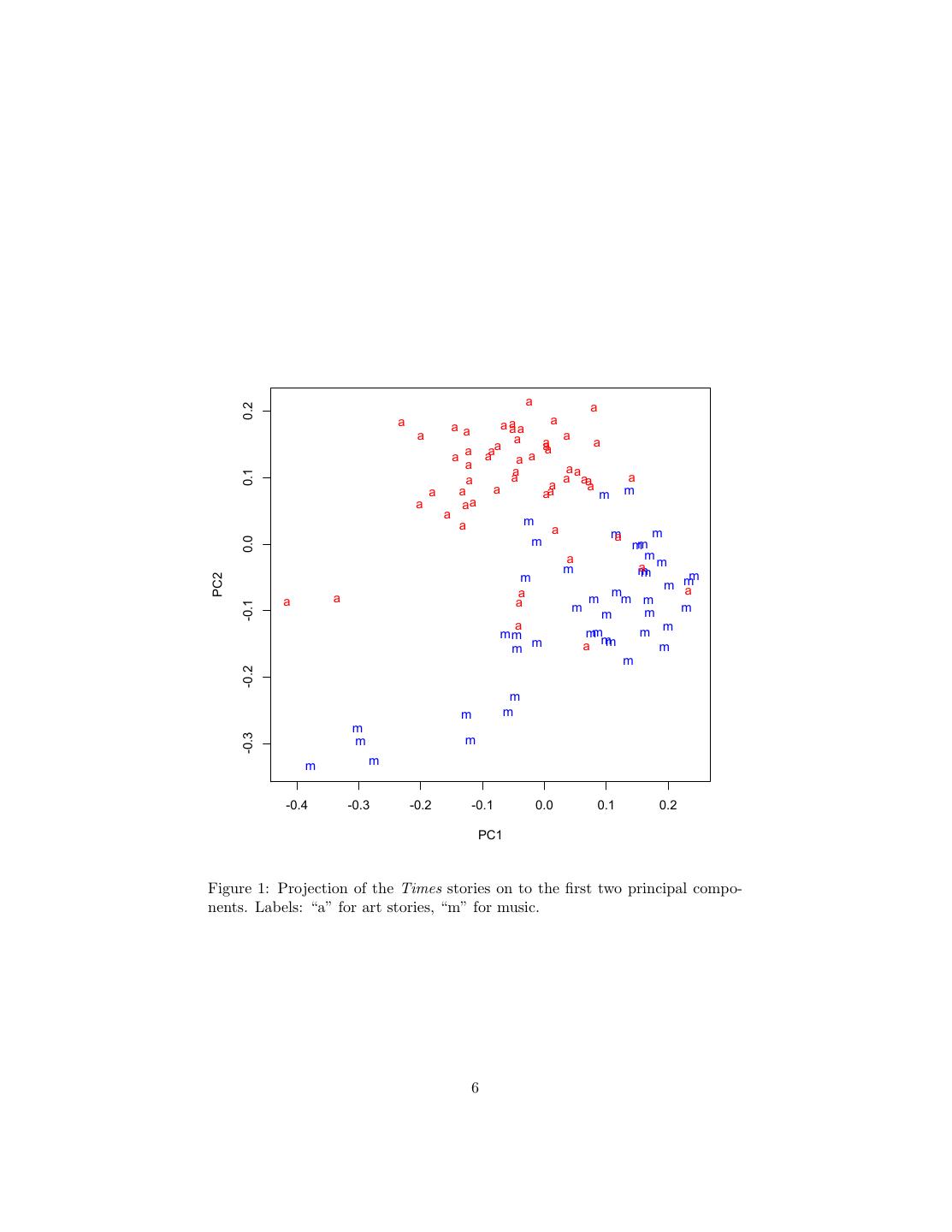
5 . play broadway singer cooper performances -0.056 -0.055 -0.052 -0.051 -0.051 Here the positive words are about art, but more focused on acquiring and trading (“collections”, “dealers”, “donations”, “dealers”) than on talking with artists or about them. The negative words are musical, specifically about musical theater and vocal performances. I could go on, but by this point you get the idea. 2 PCA for Visualization Let’s try displaying the Times stories using the principal components. (Assume that the objects from just before are still in memory.) plot(nyt.pca$x[,1:2],type="n") points(nyt.pca$x[nyt.frame[,1]=="music",1:2],pch="m",col="blue") points(nyt.pca$x[nyt.frame[,1]=="art",1:2],pch="a",col="red") The first command makes an empty plot — I do this just to set up the axes nicely for the data which will actually be displayed. The second and third commands plot a blue “m” at the location of each music story, and a red “a” at the location of each art story. The result is Figure 1. This figure should look vaguely familiar. It is basically identical to figure 2b from Lecture 2, only there I didn’t use different letters for the two classes, just different colors. How can this be? Remember that back in Lecture 2 we talked about multidimensional scal- ing, the idea of finding low-dimensional points to represent high-dimensional data by preserving the distances between the points. If we write the original vectors as x1 , x2 , . . . xn , and their images as y1 , y2 , . . . yn , then the desideratum was to minimize the difference in distances: 2 ( yi − yj − x i − x j ) i j=i This will be small if distances between the images are all close to the distances between the original points. PCA accomplishes this precisely because, as we saw last time, yi is itself close to xi (on average). References Deerwester, Scott, Susan T. Dumais, George W. Furnas, Thomas K. Lan- dauer and Richard Harshman (1990). “Indexing by Latent Semantic Analysis.” Journal of the American Society for Information Science, 41: 391–407. URL http://lsa.colorado.edu/papers/JASIS.lsi.90.pdf. doi:10.1002/(SICI)1097-4571(199009)41:6¡391::AID-ASI1¿3.0.CO;2-9. 5 

6 . a a 0.2 a a a aa a aa a a a a a aa a a a a a a a a a aa 0.1 a a a aa a a a a a a aa m m a aa a a m a m m m a 0.0 mm a m m am m m m m PC2 m m a a a m a a m m m -0.1 m m m m a m m mm mm m m a mm m m -0.2 m m m m -0.3 m m m m -0.4 -0.3 -0.2 -0.1 0.0 0.1 0.2 PC1 Figure 1: Projection of the Times stories on to the first two principal compo- nents. Labels: “a” for art stories, “m” for music. 6 

7 .Landauer, Thomas K. and Susan T. Dumais (1997). “A Solution to Plato’s Problem: The Latent Semantic Analysis Theory of Acquisition, Induction, and Representation of Knowledge.” Psychological Review , 104: 211–240. URL http://lsa.colorado.edu/papers/plato/plato.annote.html. Spearman, Charles (1904). ““General Intelligence,” Objectively Determined and Measured.” American Journal of Psychology, 15: 201–293. URL http: //psychclassics.yorku.ca/Spearman/. Thurstone, L. L. (1934). “The Vectors of Mind.” Psychological Review , 41: 1–32. URL http://psychclassics.yorku.ca/Thurstone/. 7