因子分析

1 . Factor Analysis 36-350, Data Mining 23 September 2009 Contents 1 From Principal Components to Factor Analysis 1 1.1 Measurement Error . . . . . . . . . . . . . . . . . . . . . . . . . . 1 1.2 Preserving correlations . . . . . . . . . . . . . . . . . . . . . . . . 2 1.3 Roots of Factor Analysis in Causal Discovery . . . . . . . . . . . 3 2 Preliminaries to Factor Estimation 4 3 Estimation by Linear Algebra 5 3.1 A Clue from Spearman’s One-Factor Model . . . . . . . . . . . . 5 3.2 Estimating Factor Loadings and Specific Variances . . . . . . . . 6 4 Maximum Likelihood Estimation 7 4.1 Estimating Factor Scores . . . . . . . . . . . . . . . . . . . . . . 8 5 The Rotation Problem 8 1 From Principal Components to Factor Analy- sis There are two ways to go from principal components analysis to factor analysis — two motivating stories. 1.1 Measurement Error Suppose that the numbers we write down as our observations aren’t altogether accurate — that our numbers are the true variables plus some measurement noise. (Or, if we’re not making the measurements ourselves but just taking numbers from some database, that whoever created the database wasn’t able to measure things perfectly.) PCA doesn’t care about this — it will try to reproduce true-value-plus-noise from a small number of components. But that’s 1 

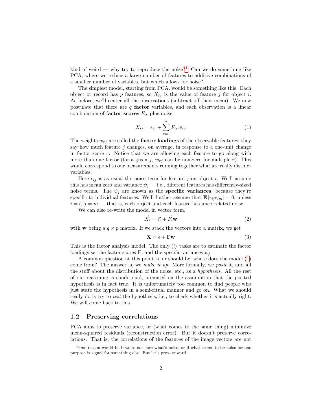
2 .kind of weird — why try to reproduce the noise?1 Can we do something like PCA, where we reduce a large number of features to additive combinations of a smaller number of variables, but which allows for noise? The simplest model, starting from PCA, would be something like this. Each object or record has p features, so Xij is the value of feature j for object i. As before, we’ll center all the observations (subtract off their mean). We now postulate that there are q factor variables, and each observation is a linear combination of factor scores Fir plus noise: k Xij = ij + Fir wrj (1) r=1 The weights wrj are called the factor loadings of the observable features; they say how much feature j changes, on average, in response to a one-unit change in factor score r. Notice that we are allowing each feature to go along with more than one factor (for a given j, wrj can be non-zero for multiple r). This would correspond to our measurements running together what are really distinct variables. Here ij is as usual the noise term for feature j on object i. We’ll assume this has mean zero and variance ψj — i.e., different features has differently-sized noise terms. The ψj are known as the specific variances, because they’re specific to individual features. We’ll further assume that E [ ij lm ] = 0, unless i = l, j = m — that is, each object and each feature has uncorrelated noise. We can also re-write the model in vector form, Xi = i + Fi w (2) with w being a q × p matrix. If we stack the vectors into a matrix, we get X = + Fw (3) This is the factor analysis model. The only (!) tasks are to estimate the factor loadings w, the factor scores F, and the specific variances ψj . A common question at this point is, or should be, where does the model (1) come from? The answer is, we make it up. More formally, we posit it, and all the stuff about the distribution of the noise, etc., as a hypothesis. All the rest of our reasoning is conditional, premised on the assumption that the posited hypothesis is in fact true. It is unfortunately too common to find people who just state the hypothesis in a semi-ritual manner and go on. What we should really do is try to test the hypothesis, i.e., to check whether it’s actually right. We will come back to this. 1.2 Preserving correlations PCA aims to preserve variance, or (what comes to the same thing) minimize mean-squared residuals (reconstruction error). But it doesn’t preserve corre- lations. That is, the correlations of the features of the image vectors are not 1 One reason would be if we’re not sure what’s noise, or if what seems to be noise for one purpose is signal for something else. But let’s press onward. 2 

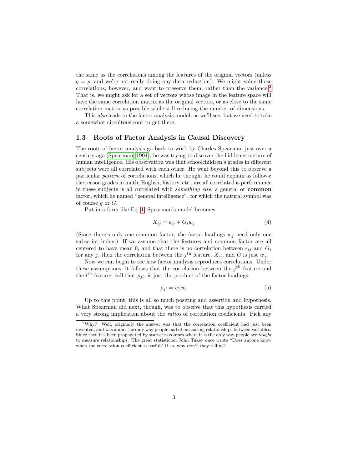
3 .the same as the correlations among the features of the original vectors (unless q = p, and we’re not really doing any data reduction). We might value those correlations, however, and want to preserve them, rather than the variance.2 That is, we might ask for a set of vectors whose image in the feature space will have the same correlation matrix as the original vectors, or as close to the same correlation matrix as possible while still reducing the number of dimensions. This also leads to the factor analysis model, as we’ll see, but we need to take a somewhat circuitous root to get there. 1.3 Roots of Factor Analysis in Causal Discovery The roots of factor analysis go back to work by Charles Spearman just over a century ago (Spearman, 1904); he was trying to discover the hidden structure of human intelligence. His observation was that schoolchildren’s grades in different subjects were all correlated with each other. He went beyond this to observe a particular pattern of correlations, which he thought he could explain as follows: the reason grades in math, English, history, etc., are all correlated is performance in these subjects is all correlated with something else, a general or common factor, which he named “general intelligence”, for which the natural symbol was of course g or G. Put in a form like Eq. 1, Spearman’s model becomes Xij = ij + Gi wj (4) (Since there’s only one common factor, the factor loadings wj need only one subscript index.) If we assume that the features and common factor are all centered to have mean 0, and that there is no correlation between ij and Gi for any j, then the correlation between the j th feature, X·j , and G is just wj . Now we can begin to see how factor analysis reproduces correlations. Under these assumptions, it follows that the correlation between the j th feature and the lth feature, call that ρjl , is just the product of the factor loadings: ρjl = wj wl (5) Up to this point, this is all so much positing and assertion and hypothesis. What Spearman did next, though, was to observe that this hypothesis carried a very strong implication about the ratios of correlation coefficients. Pick any 2 Why? Well, originally the answer was that the correlation coefficient had just been invented, and was about the only way people had of measuring relationships between variables. Since then it’s been propagated by statistics courses where it is the only way people are taught to measure relationships. The great statistician John Tukey once wrote “Does anyone know when the correlation coefficient is useful? If so, why don’t they tell us?” 3 

4 .four features, j, l, r, s. Then, if the model (4) is true, ρjr /ρlr wj wr /wl wr = (6) ρjs /ρls wj ws /wl ws wj /wl = (7) wj /wl = 1 (8) The relationship ρjr ρls = ρjs ρlr (9) is called the “tetrad equation”, and we will meet it again later when we consider methods for causal discovery. Spearman found that the tetrad equation held in his data on school grades (to a good approximation), and concluded that a single general factor of intelligence must exist. This was, of course, logically fallacious. Later work, using large batteries of different kinds of intelligence tests, showed that the tetrad equation does not hold in general, or more exactly that departures from it are too big to explain away as sampling noise. (Recall that the equations are about the true correlations between the variables, but we only get to see sample correlations, which are always a little off.) The response, done in an ad hoc way by Spearman and his followers, and then more systemati- cally by Thurstone, was to introduce multiple factors. This breaks the tetrad equation, but still accounts for the correlations among features by saying that features are really directly correlated with factors, and uncorrelated conditional on the factor scores.3 Thurstone’s form of factor analysis is basically the one people still use — there have been refinements, of course, but it’s mostly still his method. 2 Preliminaries to Factor Estimation Assume all the factor scores are uncorrelated with each other and have vari- ance 1; also that they are uncorrelated with the noise terms. We’ll solve the estimation problem for factor analysis by reducing it to an eigenvalue problem again. Start from the matrix form of the model, Eq. 3, which you’ll recall was X = + Fw (10) We know that XT X is a p × p matrix, in fact it’s n times the sample covariance 3 You can (and should!) read the classic “The Vectors of Mind” paper (Thurstone, 1934) online. 4 

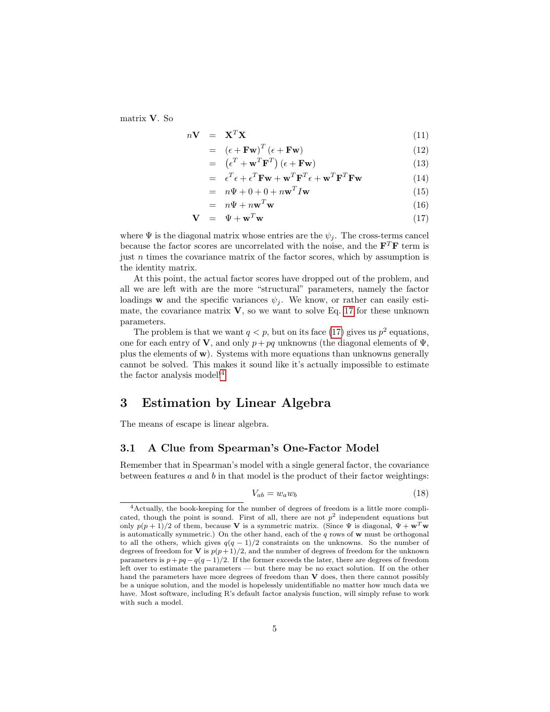
5 .matrix V. So nV = XT X (11) T = ( + Fw) ( + Fw) (12) T T T = +w F ( + Fw) (13) T T T T T T = + Fw + w F + w F Fw (14) T = nΨ + 0 + 0 + nw Iw (15) = nΨ + nwT w (16) T V = Ψ+w w (17) where Ψ is the diagonal matrix whose entries are the ψj . The cross-terms cancel because the factor scores are uncorrelated with the noise, and the FT F term is just n times the covariance matrix of the factor scores, which by assumption is the identity matrix. At this point, the actual factor scores have dropped out of the problem, and all we are left with are the more “structural” parameters, namely the factor loadings w and the specific variances ψj . We know, or rather can easily esti- mate, the covariance matrix V, so we want to solve Eq. 17 for these unknown parameters. The problem is that we want q < p, but on its face (17) gives us p2 equations, one for each entry of V, and only p + pq unknowns (the diagonal elements of Ψ, plus the elements of w). Systems with more equations than unknowns generally cannot be solved. This makes it sound like it’s actually impossible to estimate the factor analysis model!4 3 Estimation by Linear Algebra The means of escape is linear algebra. 3.1 A Clue from Spearman’s One-Factor Model Remember that in Spearman’s model with a single general factor, the covariance between features a and b in that model is the product of their factor weightings: Vab = wa wb (18) 4 Actually, the book-keeping for the number of degrees of freedom is a little more compli- cated, though the point is sound. First of all, there are not p2 independent equations but only p(p + 1)/2 of them, because V is a symmetric matrix. (Since Ψ is diagonal, Ψ + wT w is automatically symmetric.) On the other hand, each of the q rows of w must be orthogonal to all the others, which gives q(q − 1)/2 constraints on the unknowns. So the number of degrees of freedom for V is p(p + 1)/2, and the number of degrees of freedom for the unknown parameters is p + pq − q(q − 1)/2. If the former exceeds the later, there are degrees of freedom left over to estimate the parameters — but there may be no exact solution. If on the other hand the parameters have more degrees of freedom than V does, then there cannot possibly be a unique solution, and the model is hopelessly unidentifiable no matter how much data we have. Most software, including R’s default factor analysis function, will simply refuse to work with such a model. 5 

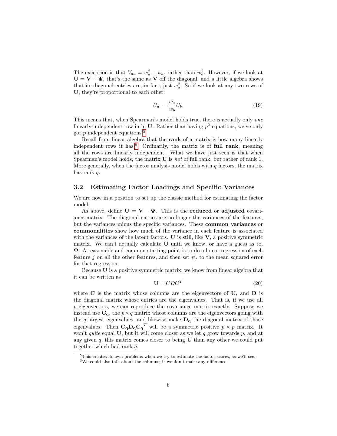
6 .The exception is that Vaa = wa2 + ψa , rather than wa2 . However, if we look at U = V − Ψ, that’s the same as V off the diagonal, and a little algebra shows that its diagonal entries are, in fact, just wa2 . So if we look at any two rows of U, they’re proportional to each other: wa Ua· = Ub· (19) wb This means that, when Spearman’s model holds true, there is actually only one linearly-independent row in in U. Rather than having p2 equations, we’ve only got p independent equations.5 Recall from linear algebra that the rank of a matrix is how many linearly independent rows it has.6 Ordinarily, the matrix is of full rank, meaning all the rows are linearly independent. What we have just seen is that when Spearman’s model holds, the matrix U is not of full rank, but rather of rank 1. More generally, when the factor analysis model holds with q factors, the matrix has rank q. 3.2 Estimating Factor Loadings and Specific Variances We are now in a position to set up the classic method for estimating the factor model. As above, define U = V − Ψ. This is the reduced or adjusted covari- ance matrix. The diagonal entries are no longer the variances of the features, but the variances minus the specific variances. These common variances or commonalities show how much of the variance in each feature is associated with the variances of the latent factors. U is still, like V, a positive symmetric matrix. We can’t actually calculate U until we know, or have a guess as to, Ψ. A reasonable and common starting-point is to do a linear regression of each feature j on all the other features, and then set ψj to the mean squared error for that regression. Because U is a positive symmetric matrix, we know from linear algebra that it can be written as U = CDC T (20) where C is the matrix whose columns are the eigenvectors of U, and D is the diagonal matrix whose entries are the eigenvalues. That is, if we use all p eigenvectors, we can reproduce the covariance matrix exactly. Suppose we instead use Cq , the p × q matrix whose columns are the eigenvectors going with the q largest eigenvalues, and likewise make Dq the diagonal matrix of those eigenvalues. Then Cq Dq Cq T will be a symmetric positive p × p matrix. It won’t quite equal U, but it will come closer as we let q grow towards p, and at any given q, this matrix comes closer to being U than any other we could put together which had rank q. 5 This creates its own problems when we try to estimate the factor scores, as we’ll see. 6 We could also talk about the columns; it wouldn’t make any difference. 6 

7 . Now define Dq 1/2 as the q × q diagonal matrix of the square roots of the eigenvalues. Clearly Dq = Dq 1/2 Dq 1/2 . So T Cq Dq Cq T = Cq Dq 1/2 Dq 1/2 Cq T = Cq Dq 1/2 Cq Dq 1/2 (21) So we have T U ≈ Cq Dq 1/2 Cq Dq 1/2 (22) but at the same time we know that U = wT w. So first we identify w with T Cq Dq 1/2 : T w = Cq Dq 1/2 (23) Now we use w to re-set Ψ, so as to fix the diagonal entries of the covariance matrix. T w = Cq Dq 1/2 (24) k 2 ψj = Vjj − wrj (25) r=1 V ≈ V ≡ Ψ + wT w (26) The “predicted” covariance matrix V in the last line is exactly right on the diagonal (by construction), and should be closer off-diagonal than anything else we could do with the same number of factors — i.e., the same rank for the U matrix. However, our estimate of U itself has in general changed, so we can try iterating this (i.e., re-calculating Cq and Dq ), until nothing changes. Let’s think a bit more about how well we’re approximating V. The approx- imation will always be exact when q = p, so that there is one factor for each feature (in which case Ψ = 0 always). Then all factor analysis does for us is to rotate the coordinate axes in feature space, so that the new coordinates are uncorrelated. (This is the same was what PCA does with p components.) The approximation can also be exact with fewer factors than features if the reduced covariance matrix is of less than full rank, and we use at least as many factors as the rank. 4 Maximum Likelihood Estimation It has probably not escaped your notice that the estimation procedure above requires a starting guess as to Ψ. This makes its consistency somewhat shaky. (If we continually put in ridiculous values for Ψ, there’s no reason to expect that w → w, even with immensely large samples.) On the other hand, we know from our elementary statistics courses that maximum likelihood estimates are generally consistent, unless we choose a spectacularly bad model. Can we use that here? 7 

8 . We can, but at a cost. We have so far got away with just making assumptions about the means and covariances of the factor scores F. To get an actual likelihood, we need to assume something about their distribution as well. The usual assumption is that Fir ∼ N (0, 1), and that the factor scores are independent across factors r = 1, . . . q and individuals i = 1, . . . n. With this assumption, the features have a multivariate normal distribution Xi ∼ N (0, Ψ + wT w). This means that the log-likelihood is np n n −1 L=− log 2π − log |Ψ + wT w| − tr (Ψ + wT w) V (27) 2 2 2 where tr A is the trace of the matrix A, the sum of its diagonal elements. One can either try direct numerical maximization, or use a two-stage pro- cedure. Starting, once again, with a guess as to Ψ, one finds that the optimal choice of Ψ1/2 wT is given by the matrix whose columns are the q leading eigen- vectors of Ψ1/2 VΨ1/2 . Starting from a guess as to w, the optimal choice of Ψ is given by the diagonal entries of V − wT w. So again one starts with a guess about the unique variances (e.g., the residuals of the regressions) and iterates to convergence.7 The differences between the maximum likelihood estimates and the “prin- cipal factors” approach can be substantial. If the data appear to be normally distributed (as shown by the usual tests), then the additional efficiency of max- imum likelihood estimation is highly worthwhile. Also, as we’ll see next time, it is a lot easier to test the model assumptions is one uses the MLE. 4.1 Estimating Factor Scores The probably the best method for estimating factor scores is the “regression” or “Thomson” method, which says Fir = Xij bij (28) j and seeks the weights bij which will minimize the mean squared error, E[(Fir − Fir )2 ]. You will see how this works in a homework problem. 5 The Rotation Problem Recall from linear algebra that a matrix O is orthogonal if its inverse is the same as its transpose, OT O = I. The classic examples are rotation matrices. For instance, to rotate a two-dimensional vector through an angle α, we multiply it by cos α − sin α Rα = (29) sin α cos α 7 The algebra is tedious. See section 3.2 in Bartholomew (1987) if you really want it. (Note that Bartholomew has a sign error in his equation 3.16.) 8 

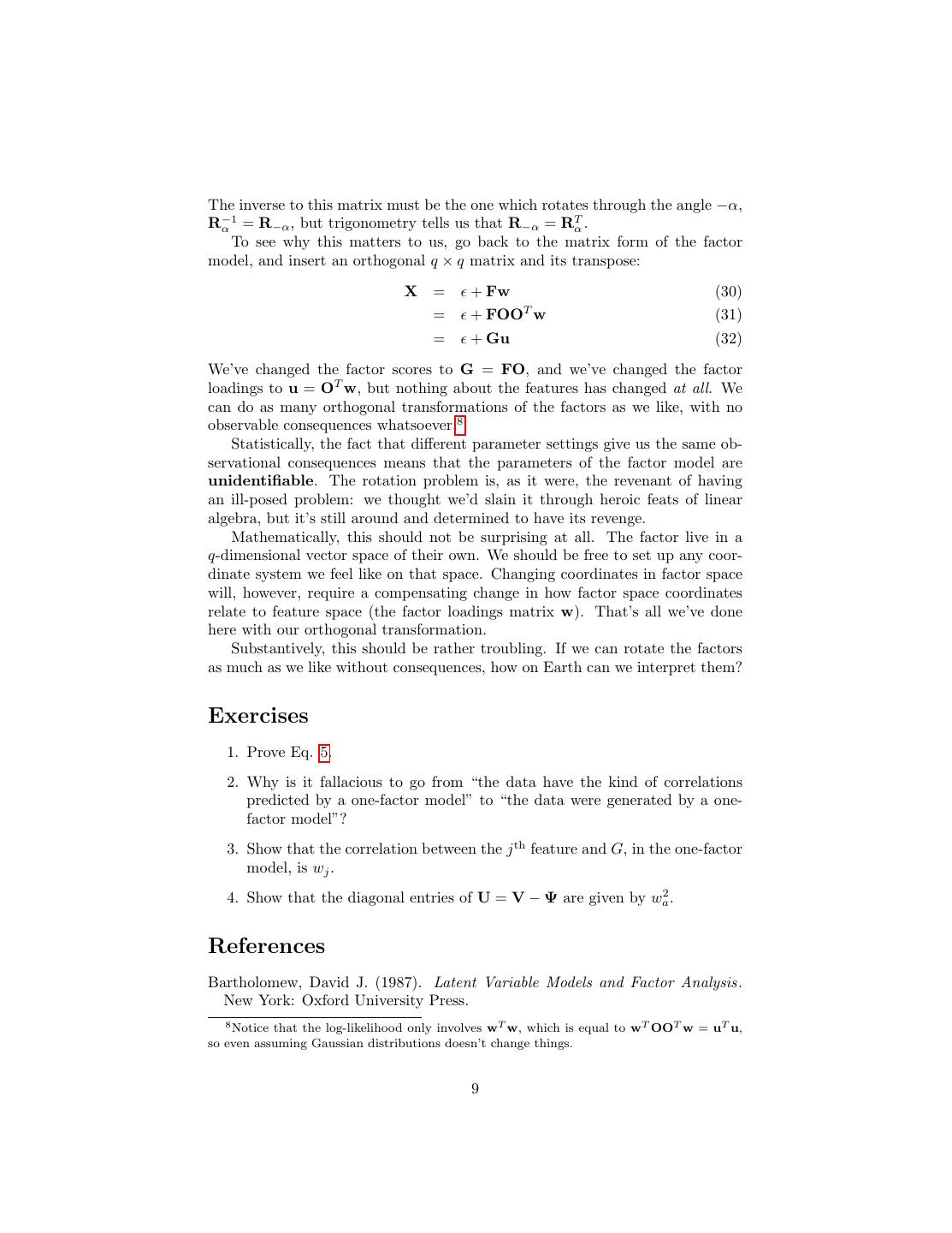
9 .The inverse to this matrix must be the one which rotates through the angle −α, R−1 α = R−α , but trigonometry tells us that R−α = Rα . T To see why this matters to us, go back to the matrix form of the factor model, and insert an orthogonal q × q matrix and its transpose: X = + Fw (30) T = + FOO w (31) = + Gu (32) We’ve changed the factor scores to G = FO, and we’ve changed the factor loadings to u = OT w, but nothing about the features has changed at all. We can do as many orthogonal transformations of the factors as we like, with no observable consequences whatsoever.8 Statistically, the fact that different parameter settings give us the same ob- servational consequences means that the parameters of the factor model are unidentifiable. The rotation problem is, as it were, the revenant of having an ill-posed problem: we thought we’d slain it through heroic feats of linear algebra, but it’s still around and determined to have its revenge. Mathematically, this should not be surprising at all. The factor live in a q-dimensional vector space of their own. We should be free to set up any coor- dinate system we feel like on that space. Changing coordinates in factor space will, however, require a compensating change in how factor space coordinates relate to feature space (the factor loadings matrix w). That’s all we’ve done here with our orthogonal transformation. Substantively, this should be rather troubling. If we can rotate the factors as much as we like without consequences, how on Earth can we interpret them? Exercises 1. Prove Eq. 5. 2. Why is it fallacious to go from “the data have the kind of correlations predicted by a one-factor model” to “the data were generated by a one- factor model”? 3. Show that the correlation between the j th feature and G, in the one-factor model, is wj . 4. Show that the diagonal entries of U = V − Ψ are given by wa2 . References Bartholomew, David J. (1987). Latent Variable Models and Factor Analysis. New York: Oxford University Press. 8 Notice that the log-likelihood only involves wT w, which is equal to wT OOT w = uT u, so even assuming Gaussian distributions doesn’t change things. 9 

10 .Spearman, Charles (1904). ““General Intelligence,” Objectively Determined and Measured.” American Journal of Psychology, 15: 201–293. URL http: //psychclassics.yorku.ca/Spearman/. Thurstone, L. L. (1934). “The Vectors of Mind.” Psychological Review , 41: 1–32. URL http://psychclassics.yorku.ca/Thurstone/. 10