聚类II

1 . Distances between Clustering, Hierarchical Clustering 36-350, Data Mining 14 September 2009 Contents 1 Distances Between Partitions 1 2 Hierarchical clustering 2 2.1 Ward’s method . . . . . . . . . . . . . . . . . . . . . . . . . . . . 3 2.1.1 Picking the Number of Clusters . . . . . . . . . . . . . . . 3 2.1.2 Ward’s Method in Action . . . . . . . . . . . . . . . . . . 4 2.2 Single-link Clustering . . . . . . . . . . . . . . . . . . . . . . . . 4 2.3 Complete-Link Clustering . . . . . . . . . . . . . . . . . . . . . . 4 3 How Many Clusters? 4 4 Reification 8 1 Distances Between Partitions Different clustering algorithms will give us different results on the same data. The same clustering algorithm may give us different results on the same data, if, like k-means, it involves some arbitrary initial condition. We would like to say how far apart two clusterings of the same data are. In doing this, we want to accommodate different numbers of clusters, and we want to accommodate the fact that cluster labels are completely arbitrary, so we want to say two clusterings are the same if they only differ by the labels. Recall that a partition of a set divides it into subsets where are mutu- ally exclusive (no point in the set is in more than one subset) and jointly exhaustive (every point is in some subset). The subsets are called the cells of the partition. When we have class labels, the classes partition the data. What we get from a clustering procedure is another partition. Whenever we have two partitions of the same data, we can build a confusion matrix, just as we did for classifiers; call it A. The entry Aij is the number of items which are in cell i of the first partition and cell j of the second partition. 1 

2 .When we did this for classifiers, the first partition was that of the true classes, and the second partition was that of our guesses; we wanted the diagonal entries of A to be big and the rest small, because that meant we were guessing correctly. Two clusterings can be close, however, even if the diagonal isn’t, because the numbering of the clusters is essentially arbitrary. One distance measure which does what we want — which is invariant under permutations of the cluster labels — is what’s called the variation of infor- mation metric.1 Pick a point from the set completely at random, and let X be the cell it falls into according to the first partition, and Y its cell in the second partition. Then the distance is H[X|Y ] + H[Y |X] (1) This will be zero if and only if there is a 1-1 correspondence between the cells of the two partitions. Otherwise, it will be positive, and the larger it is, the less information we get about one partition from the other. (Its maximum possible value is H[X] + H[Y ].) 2 Hierarchical clustering The k-means algorithm gives us what’s sometimes called a simple or flat par- tition, because it just gives us a single set of clusters, with no particular orga- nization or structure within them. But it could easily be the case that some clusters could, themselves, be closely related to other clusters, and more dis- tantly related to others. (If we are clustering images, we might want not just to have a cluster of flowers, but roses and marigolds within that. Or, if we’re clustering patient medical records, we might want “respiratory complaints” as a super-cluster of “pneumonia”, “influenza”, “SARS”, “miscellaneous sniffling”.) So sometimes we want a hierarchical clustering, which is depicted by a tree or dendrogram. There are two approaches to hierarchical clustering: we can go “from the bottom up”, grouping small clusters into larger ones, or “from the top down”, splitting big clusters into small ones. These are called agglomerative and divisive clusterings, respectively. We will return to divisive clustering later, after we have tools to talk about the over-all pattern of connections among data points. For today, we’ll stick to agglomerative clustering. The basic algorithm is very simple: 1. Start with each point in a cluster of its own 2. Until there is only one cluster (a) Find the closest pair of clusters (b) Merge them 1 It has many names, actually. 2 

3 . 3. Return the tree of cluster-mergers Any such procedure is greedy, like our feature-selection algorithm and deter- ministic (no random initial conditions, unlike k-means). It returns a sequence of nested partitions, where each level up merges two cells of the lower partition.2 To turn this into a definite procedure, though, we need to be able to say how close two clusters are. This is not the same as how close two data points are, or how close two partitions are. There are three basic choices, and a lot of wrinkles. 2.1 Ward’s method Ward’s method says that the distance between two clusters, A and B, is how much the sum of squares will increase when we merge them: 2 2 2 ∆(A, B) = xi − mA∪B − xi − mA − xi − mB (2) i∈A∪B i∈A i∈B nA nB 2 = mA − mB (3) nA + nB where mj is the center of cluster j, and nj is the number of points in it. ∆ is called the merging cost of combining the clusters A and B. With hierarchical clustering, the sum of squares starts out at zero (because every point is in its own cluster) and then grows as we merge clusters. Ward’s method keeps this growth as small as possible. This is nice if you believe that the sum of squares should be small. Notice that the number of points shows up in ∆, as well as their geometric separation. Given two pairs of clusters whose centers are equally far apart, Ward’s method will prefer to merge the smaller ones. Ward’s method is both greedy, and constrained by previous choices as to which clusters to form. This means its sum-of-squares for a given number k of clusters is usually larger than the minimum for that k, and even larger than what k-means will achieve. If this is bothersome for your application, one common trick is use hierarchical clustering to pick k (see below), and then run k-means starting from the clusters found by Ward’s method to reduce the sum of squares from a good starting point. 2.1.1 Picking the Number of Clusters The k-means algorithm gives no guidance about what k should be. Ward’s algorithm, on the other hand, can give us a hint through the merging cost. If the cost of merging increases a lot, it’s probably going too far, and losing a lot of structure. So a rule of thumb is to keep reducing k until the cost jumps, and then use the k right before the jump. Of course this leaves you to decide how big a merging cost is acceptable, and there’s no theory whatsoever to say that 2 We say that one partition is finer than another, or is a refinement of it, if every cell of the finer partition is contained within some cell of the coarser partition. Hierarchical clustering gives us a sequence of increasingly fine partitions. 3 

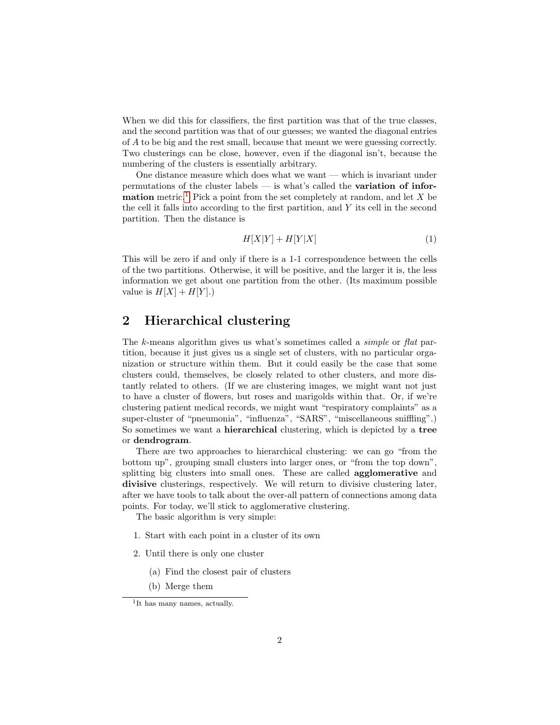
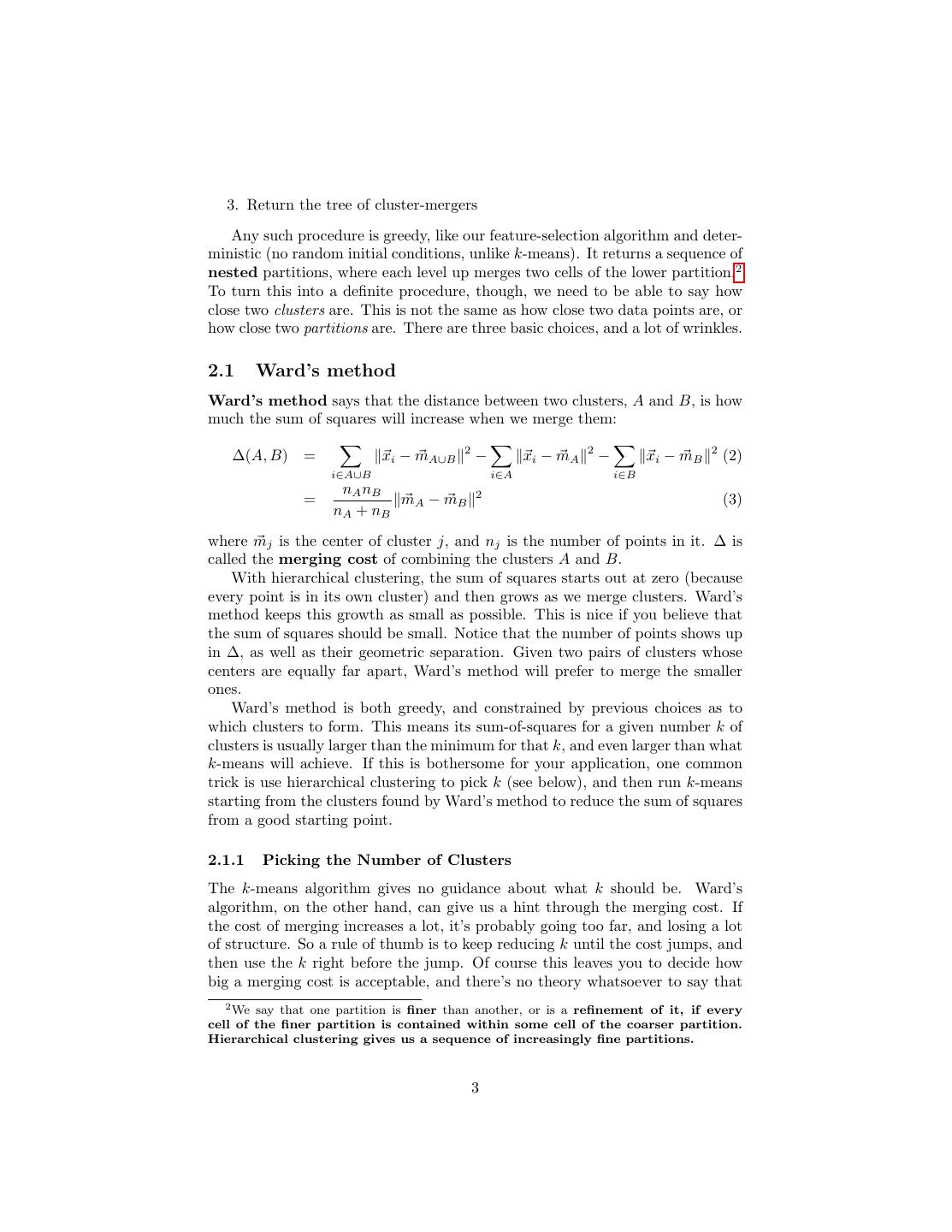
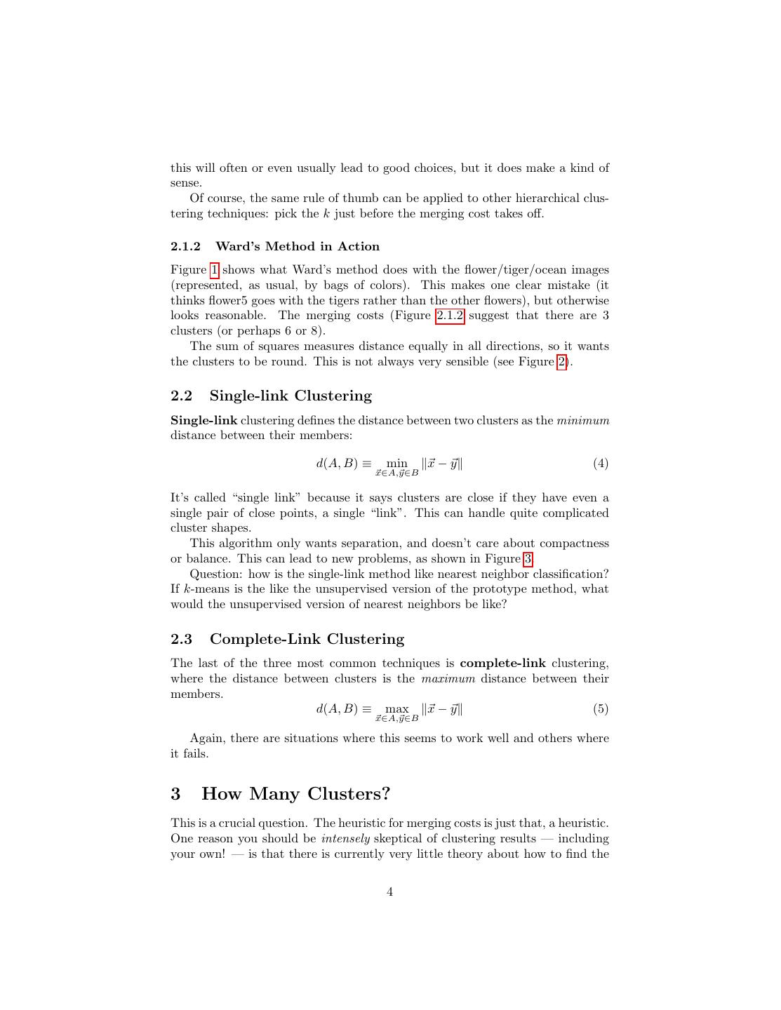
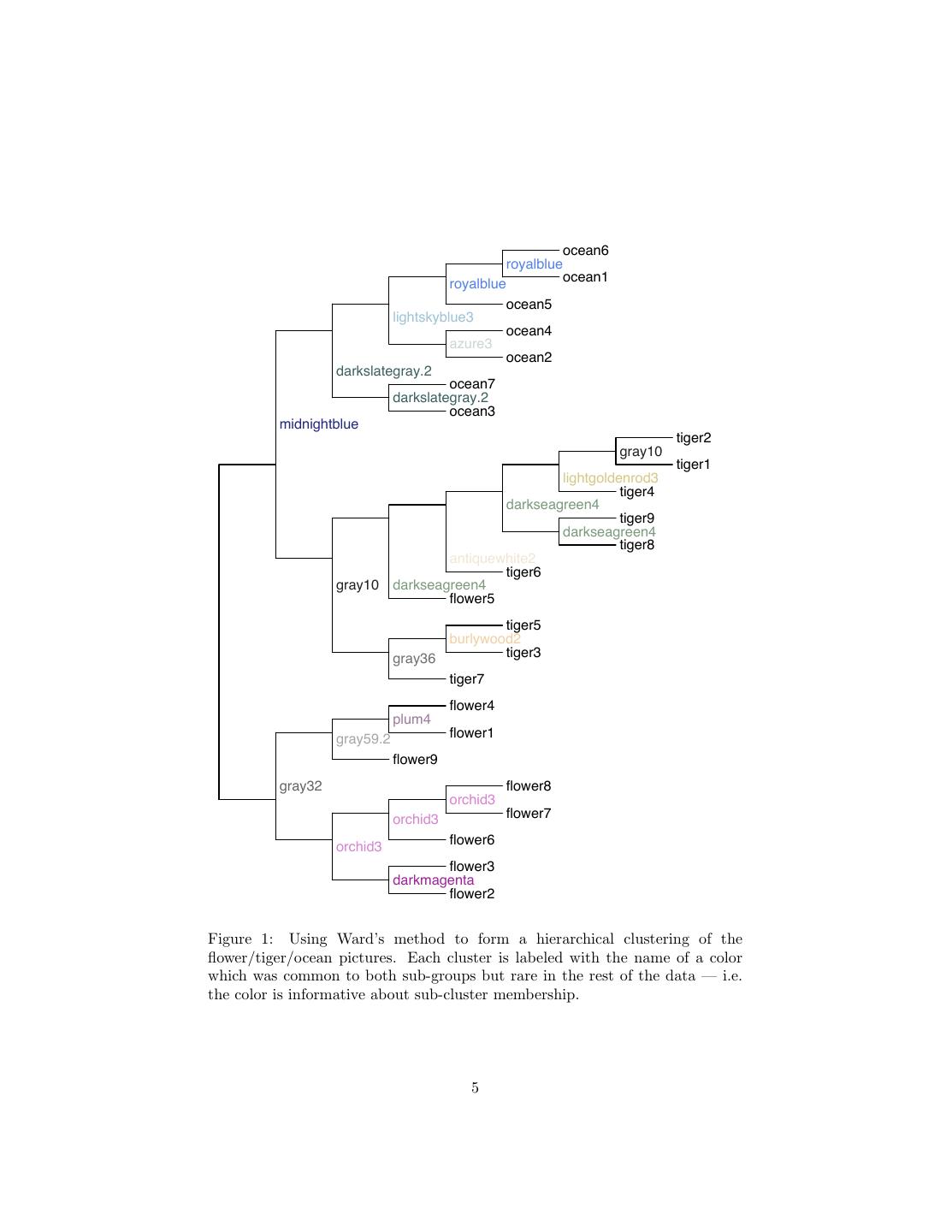
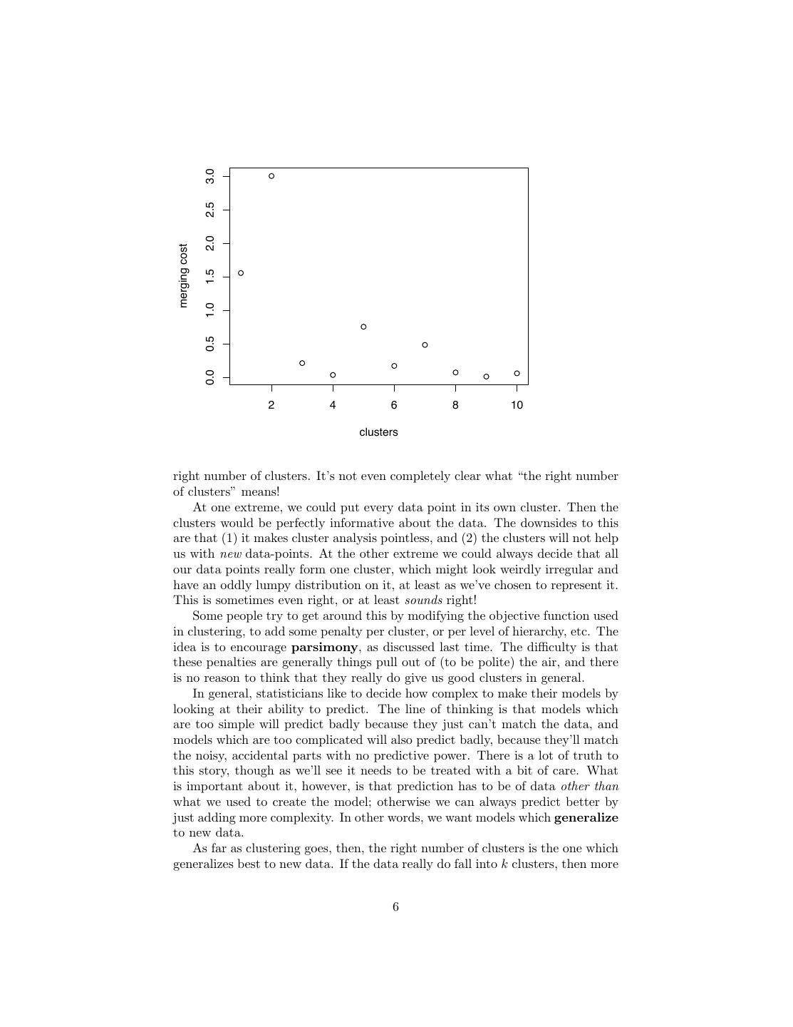
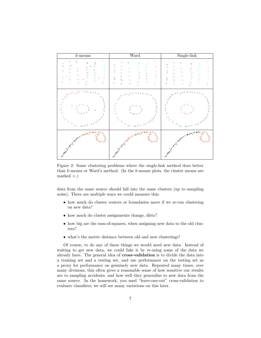
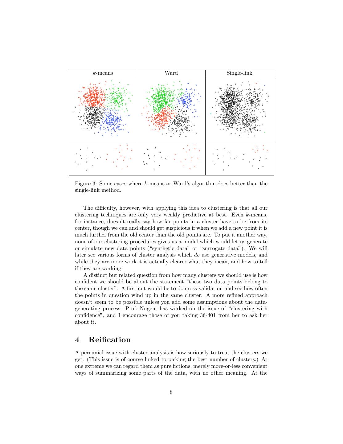
4 .this will often or even usually lead to good choices, but it does make a kind of sense. Of course, the same rule of thumb can be applied to other hierarchical clus- tering techniques: pick the k just before the merging cost takes off. 2.1.2 Ward’s Method in Action Figure 1 shows what Ward’s method does with the flower/tiger/ocean images (represented, as usual, by bags of colors). This makes one clear mistake (it thinks flower5 goes with the tigers rather than the other flowers), but otherwise looks reasonable. The merging costs (Figure 2.1.2 suggest that there are 3 clusters (or perhaps 6 or 8). The sum of squares measures distance equally in all directions, so it wants the clusters to be round. This is not always very sensible (see Figure 2). 2.2 Single-link Clustering Single-link clustering defines the distance between two clusters as the minimum distance between their members: d(A, B) ≡ min x−y (4) x∈A,y∈B It’s called “single link” because it says clusters are close if they have even a single pair of close points, a single “link”. This can handle quite complicated cluster shapes. This algorithm only wants separation, and doesn’t care about compactness or balance. This can lead to new problems, as shown in Figure 3. Question: how is the single-link method like nearest neighbor classification? If k-means is the like the unsupervised version of the prototype method, what would the unsupervised version of nearest neighbors be like? 2.3 Complete-Link Clustering The last of the three most common techniques is complete-link clustering, where the distance between clusters is the maximum distance between their members. d(A, B) ≡ max x − y (5) x∈A,y∈B Again, there are situations where this seems to work well and others where it fails. 3 How Many Clusters? This is a crucial question. The heuristic for merging costs is just that, a heuristic. One reason you should be intensely skeptical of clustering results — including your own! — is that there is currently very little theory about how to find the 4 

5 . ocean6 royalblue royalblue ocean1 ocean5 lightskyblue3 ocean4 azure3 ocean2 darkslategray.2 ocean7 darkslategray.2 ocean3 midnightblue tiger2 gray10 tiger1 lightgoldenrod3 tiger4 darkseagreen4 tiger9 darkseagreen4 tiger8 antiquewhite2 tiger6 gray10 darkseagreen4 flower5 tiger5 burlywood2 gray36 tiger3 tiger7 flower4 plum4 gray59.2 flower1 flower9 gray32 flower8 orchid3 orchid3 flower7 orchid3 flower6 flower3 darkmagenta flower2 Figure 1: Using Ward’s method to form a hierarchical clustering of the flower/tiger/ocean pictures. Each cluster is labeled with the name of a color which was common to both sub-groups but rare in the rest of the data — i.e. the color is informative about sub-cluster membership. 5 

6 . 3.0 2.5 2.0 merging cost 1.5 1.0 0.5 0.0 2 4 6 8 10 clusters right number of clusters. It’s not even completely clear what “the right number of clusters” means! At one extreme, we could put every data point in its own cluster. Then the clusters would be perfectly informative about the data. The downsides to this are that (1) it makes cluster analysis pointless, and (2) the clusters will not help us with new data-points. At the other extreme we could always decide that all our data points really form one cluster, which might look weirdly irregular and have an oddly lumpy distribution on it, at least as we’ve chosen to represent it. This is sometimes even right, or at least sounds right! Some people try to get around this by modifying the objective function used in clustering, to add some penalty per cluster, or per level of hierarchy, etc. The idea is to encourage parsimony, as discussed last time. The difficulty is that these penalties are generally things pull out of (to be polite) the air, and there is no reason to think that they really do give us good clusters in general. In general, statisticians like to decide how complex to make their models by looking at their ability to predict. The line of thinking is that models which are too simple will predict badly because they just can’t match the data, and models which are too complicated will also predict badly, because they’ll match the noisy, accidental parts with no predictive power. There is a lot of truth to this story, though as we’ll see it needs to be treated with a bit of care. What is important about it, however, is that prediction has to be of data other than what we used to create the model; otherwise we can always predict better by just adding more complexity. In other words, we want models which generalize to new data. As far as clustering goes, then, the right number of clusters is the one which generalizes best to new data. If the data really do fall into k clusters, then more 6 

7 . k-means Ward Single-link Figure 2: Some clustering problems where the single-link method does better than k-means or Ward’s method. (In the k-means plots, the cluster means are marked ×.) data from the same source should fall into the same clusters (up to sampling noise). There are multiple ways we could measure this: • how much do cluster centers or boundaries move if we re-run clustering on new data? • how much do cluster assignments change, ditto? • how big are the sum-of-squares, when assigning new data to the old clus- ters? • what’s the metric distance between old and new clusterings? Of course, to do any of these things we would need new data. Instead of waiting to get new data, we could fake it by re-using some of the data we already have. The general idea of cross-validation is to divide the data into a training set and a testing set, and use performance on the testing set as a proxy for performance on genuinely new data. Repeated many times, over many divisions, this often gives a reasonable sense of how sensitive our results are to sampling accidents, and how well they generalize to new data from the same source. In the homework, you used “leave-one-out” cross-validation to evaluate classifiers; we will see many variations on this later. 7 

8 . k-means Ward Single-link Figure 3: Some cases where k-means or Ward’s algorithm does better than the single-link method. The difficulty, however, with applying this idea to clustering is that all our clustering techniques are only very weakly predictive at best. Even k-means, for instance, doesn’t really say how far points in a cluster have to be from its center, though we can and should get suspicious if when we add a new point it is much further from the old center than the old points are. To put it another way, none of our clustering procedures gives us a model which would let us generate or simulate new data points (“synthetic data” or “surrogate data”). We will later see various forms of cluster analysis which do use generative models, and while they are more work it is actually clearer what they mean, and how to tell if they are working. A distinct but related question from how many clusters we should use is how confident we should be about the statement “these two data points belong to the same cluster”. A first cut would be to do cross-validation and see how often the points in question wind up in the same cluster. A more refined approach doesn’t seem to be possible unless you add some assumptions about the data- generating process. Prof. Nugent has worked on the issue of “clustering with confidence”, and I encourage those of you taking 36-401 from her to ask her about it. 4 Reification A perennial issue with cluster analysis is how seriously to treat the clusters we get. (This issue is of course linked to picking the best number of clusters.) At one extreme we can regard them as pure fictions, merely more-or-less convenient ways of summarizing some parts of the data, with no other meaning. At the 8 

9 .other end we can insist that they reflect real divisions of the world into distinct types. This is an instance of the general problem of how seriously to take our theoretical constructs — of when and whether they should be reified, made into things. This is especially tempting once we have attached meaningful names to clusters (as opposed to just calling them “cluster 1”, “cluster 2”, . . . “cluster k”). On the one hand, there are some theoretical constructs which it is absurd not to believe are real: germs and atoms, for instance. On the other hand, we do not think that constellations have any reality or meaning beyond giving convenient ways of dividing up the sky.3 How can we tell when our clusters are more like bacteria and when they are more like the signs of the zodiac? A full answer is beyond the scope of this class (not least because nobody has a full answer). I can however point to three things which seem more or less compelling. 1. Good clusters should generalize well. We talked about this above; to reca- pitulate briefly, the clusters should continue to describe new observations of the same features. 2. Good clusters should generalize to new features. Knowing someone’s as- trological sign predicts nothing else about them. On other hand, if we identify a bird’s species from its bodily shape, that predicts many other attributes: its coloration, its song, when it mates, whether and where it migrates, what it eats, its genome, etc. Bird species, then, is a good cluster. 3. Good clusters should fit into a theory, they should be a part of a valid system of generalizations which lets us make predictions about new con- ditions, and explains why things turn out the way they do. The first of these seems like a basic requirement before we should even bother with a clustering. The second is considerably stricter, but it needs to be dealt with cautiously, since clusters don’t have to be relevant for everything in order to be valid. Finally, while being part of a well-established theory is a great thing, it’s honestly pretty rare in most situations where people think to look for clusters in the first place. The lack of good theoretical checks, of course, also makes it all the more tempting to reify clusters. Paul (2004) provides an entertain account of how psychologists have embraced this temptation when it comes to personality types, and I strongly encourage you to read it. Demographics, especially as applied to politics and marketing, is another prime offender. You should look at both http://yawyl.claritas.com and http://www.inthesetimes.com/article/ 3320/trending_towards_inanity/; for the former your job is to figure out what they are doing, and for the latter to figure out what Penn is doing and avoid it. 3 Of course for thousands of years all the most learned people in the world thought otherwise. 9 

10 .References Paul, Annie Murphy (2004). The Cult of Personality: How Personality Tests Are Leading Us to Miseducate Our Children, Mismanage Our Companies, and Misunderstand Ourselves. New York: Free Press. 10