The Truth About Linear Regression

1 . The Truth About Linear Regression 36-350, Data Mining 21 October 2009 Contents 1 Optimal Linear Prediction 2 1.1 Collinearity . . . . . . . . . . . . . . . . . . . . . . . . . . . . . . 3 1.2 Estimating the Optimal Linear Predictor . . . . . . . . . . . . . 3 2 Shifting Distributions, Omitted Variables, and Transformations 4 2.1 Changing Slopes . . . . . . . . . . . . . . . . . . . . . . . . . . . 4 2.1.1 R2 : Distraction or Nuisance? . . . . . . . . . . . . . . . . 6 2.2 Omitted Variables and Shifting Distributions . . . . . . . . . . . 6 2.3 Errors in Variables . . . . . . . . . . . . . . . . . . . . . . . . . . 9 2.4 Transformation . . . . . . . . . . . . . . . . . . . . . . . . . . . . 11 3 Adding Probabilistic Assumptions 14 3.1 Examine the Residuals . . . . . . . . . . . . . . . . . . . . . . . . 15 4 Linear Regression Is Not the Philosopher’s Stone 16 5 Exercises 18 A Where the χ2 Likelihood Ratio Test Comes From 19 We need to say some more about how linear regression, and especially about how it really works and how it can fail. Linear regression is important because 1. it’s a fairly straightforward technique which often works reasonably well; 2. it’s a simple foundation for some more sophisticated techniques; 3. it’s a standard method so people use it to communicate; and 4. it’s a standard method so people have come to confuse it with prediction and even with causal inference as such. We need to go over (1)–(3), and provide prophylaxis against (4). There are many good books available about linear regression. Faraway (2004) is practical and has a lot of useful R stuff. Berk (2004) omits tech- nical details, but is superb on the high-level picture, and especially on what 1 

2 .must be assumed in order to do certain things with regression, and what cannot be done under any assumption. 1 Optimal Linear Prediction We have a response variable Y and a p-dimensional vector of predictor variables or features X. To simplify the book-keeping, we’ll take these to be centered — we can always un-center them later. We would like to predict Y using X. We saw last time that the best predictor we could use, at least in a mean-squared sense, is the conditional expectation, r(x) = E Y |X = x (1) Let’s approximate r(x) by a linear function of x, say x · β. This is not an assumption about the world, but rather a decision on our part; a choice, not a hypothesis. This decision can be good — the approximation can be accurate — even if the linear hypothesis is wrong. One reason to think it’s not a crazy decision is that we may hope r is a smooth function. If it is, then we can Taylor expand it about our favorite point, say u: p ∂r 2 r(x) = r(u) + (xi − ui ) + O( x − u ) (2) i=1 ∂x i u or, in the more compact vector calculus notation, 2 r(x) = r(u) + (x − u) · ∇r(u) + O( x − u ) (3) If we only look at points x which are close to u, then the remainder terms 2 O( x − u ) are small, and a linear approximation is a good one. Of course there are lots of linear functions so we need to pick one, and we may as well do that by minimizing mean-squared error again: 2 M SE(β) = E Y −X ·β (4) Going through the optimization is parallel to the one-dimensional case (see last handout), with the conclusion that the optimal β is β = V−1 Cov X, Y (5) where V is the covariance matrix of X, i.e., Vij = Cov [Xi , Xj ], and Cov X, Y is the vector of covariances between the predictor variables and Y , i.e. Cov X, Y = i Cov [Xi , Y ]. If Z is a random vector with covariance matrix I, then VZ is a random vector with covariance matrix V. Conversely, V−1 X will be a random vector 2 

3 .with covariance matrix I. We are using the covariance matrix here to transform the input features into uncorrelated variables, then taking their correlations with the response — we are decorrelating them. Notice: β depends on the marginal distribution of X (through the covariance matrix V). If that shifts, the optimal coefficients β will shift, unless the real regression function is linear. 1.1 Collinearity The formula β = V−1 Cov X, Y makes no sense if V has no inverse. This will happen if, and only if, the predictor variables are linearly dependent on each other — if one of the predictors is really a linear combination of the others. Then (think back to what we did with factor analysis) the covariance matrix is of less than full rank (i.e., rank deficient) and it doesn’t have an inverse. So much for the algebra; what does that mean statistically? Let’s take an easy case where one of the predictors is just a multiple of the others — say you’ve included people’s weight in pounds (X1 ) and mass in kilograms (X2 ), so X1 = 2.2X2 . Then if we try to predict Y , we’d have Yˆ = β1 X1 + β2 X2 + β3 X3 + . . . + βp Xp p = 0X1 + (2.2β1 + β2 )X2 + βi Xi i=3 p = (β1 + β2 /2.2)X1 + 0X2 + βi Xi i=3 p = −2200X1 + (1000 + β1 + β2 )X2 + βi Xi i=3 In other words, because there’s a linear relationship between X1 and X2 , we make the coefficient for X1 whatever we like, provided we make a corresponding adjustment to the coefficient for X2 , and it has no effect at all on our prediction. So rather than having one optimal linear predictor, we have infinitely many of them. There are two ways of dealing with collinearity. One is to get a different data set where the predictor variables are no longer collinear. The other is to identify one of the collinear variables (it doesn’t matter which) and drop it from the data set. This can get complicated; PCA can be helpful here. 1.2 Estimating the Optimal Linear Predictor To actually estimate β, we need to make some probabilistic assumptions about where the data comes from. The minimal one we can get away with is that observations (Xi , Yi ) are independent for different values of i, with unchanging covariances. Then if we look at the sample covariances, they will converge on 3 

4 .the true covariances: 1 T X Y → Cov X, Y n 1 T X X → V n where as before X is the data-frame matrix with one row for each data point and one column for each feature, and similarly for Y. So, by continuity, −1 β = (XT X) XT Y → β (6) and we have a consistent estimator. On the other hand, we could start with the residual sum of squares n 2 RSS(β) ≡ (yi − xi · β) (7) i=1 and try to minimize it. The minimizer is the same β we got by plugging in the sample covariances. No probabilistic assumption is needed to do this, but it doesn’t let us say anything about the convergence of β. (One can also show that the least-squares estimate is the linear prediction with the minimax prediction risk. That is, its worst-case performance, when everything goes wrong and the data are horrible, will be better than any other linear method. This is some comfort, especially if you have a gloomy and pes- simistic view of data, but other methods of estimation may work better in less-than-worst-case scenarios.) 2 Shifting Distributions, Omitted Variables, and Transformations 2.1 Changing Slopes I said earlier that the best β in linear regression will depend on the distribution of the predictor variable, unless the conditional mean is exactly linear. Here is an illustration. For simplicity, let’s say √ that p = 1, so there’s only one predictor variable. I generated data from Y = X + , with ∼ N (0, 0.052 ) (i.e. the standard deviation of the noise was 0.05). Figure 1 shows the regression lines inferred from samples with three different distributions of X: the black points are X ∼ Unif(0, 1), the blue are X ∼ N (0.5, 0.01) and the red X ∼ Unif(2, 3). The regression lines are shown as colored solid lines; those from the blue and the black data are quite similar — and similarly wrong. The dashed black line is the regression line fitted to the complete√ data set. Finally, the light grey curve is the true regression function, r(x) = x. 4 

5 . 3.0 2.5 2.0 1.5 y1 1.0 0.5 0.0 0.0 0.5 1.0 1.5 2.0 2.5 3.0 x1 √ Figure 1: Behavior of the conditioning distribution Y |X ∼ N ( X, 0.052 ) with different distributions of X. Black circles: X is uniformly distributed in the unit interval. Blue triangles: Gaussian with mean 0.5 and standard deviation 0.1. Red squares: uniform between 2 and 3. Axis tick-marks show the location of the actual sample points. Solid colored lines show the three regression lines obtained by fitting to the three different data sets; the dashed line is from fitting to all three. The grey curve is the true regression function. 5 

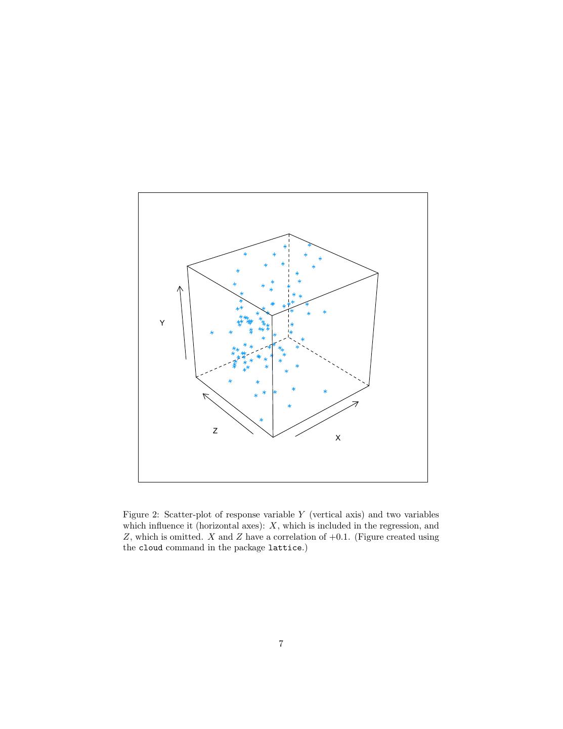
6 .2.1.1 R2 : Distraction or Nuisance? This little set-up, by the way, illustrates that R2 is not a stable property of the distribution either. For the black points, R2 = 0.92; for the blue, R2 = 0.70; and for the red, R2 = 0.77; and for the complete data, 0.96. Other sets of xi values would give other values for R2 . Note that while the global linear fit isn’t even a good approximation anywhere in particular, it has the highest R2 . This kind of perversity can happen even in a completely linear set-up. Sup- pose now that Y = aX + , and we happen to know a exactly. The variance of Y will be a2 Var [X] + Var [ ]. The amount of variance our regression “ex- plains” — really, the variance of our predictions —- will be a2 Var [X]. So a2 Var[X] R2 = a2 Var[X]+Var[ ] . This goes to zero as Var [X] → 0 and it goes to 1 as Var [X] → ∞. It thus has little to do with the quality of the fit, and a lot to do with how spread out the independent variable is. Notice also how easy it is to get a very high R2 even when the true model is not linear! 2.2 Omitted Variables and Shifting Distributions That the optimal regression coefficients can change with the distribution of the predictor features is annoying, but one could after all notice that the distribution has shifted, and so be cautious about relying on the old regression. More subtle is that the regression coefficients can depend on variables which you do not measure, and those can shift without your noticing anything. Mathematically, the issue is that E Y |X = E E Y |Z, X |X (8) Now, if Y is independent of Z given X, then the extra conditioning in the inner expectation does nothing and changing Z doesn’t alter our predictions. But in general there will be plenty of variables Z which we don’t measure (so they’re not included in X) but which have some non-redundant information about the response (so that Y depends on Z even conditional on X). If the distribution of Z given X changes, then the optimal regression of Y on X should change too. Here’s an example. X and Z are both N (0, 1), but with a positive correlation of 0.1. In reality, Y ∼ N (X + Z, 0.01). Figure 2 shows a scatterplot of all three variables together (n = 100). Now I change the correlation between X and Z to −0.1. This leaves both marginal distributions alone, and is barely detectable by eye (Figure 3).1 Figure 4 shows just the X and Y values from the two data sets, in black for the points with a positive correlation between X and Z, and in blue when the correlation is negative. Looking by eye at the points and at the axis tick- marks, one sees that, as promised, there is very little change in the marginal distribution of either variable. Furthermore, the correlation between X and Y 1 I’m sure there’s a way to get R to combine the scatterplots, but it’s beyond me. 6 

7 . Y Z X Figure 2: Scatter-plot of response variable Y (vertical axis) and two variables which influence it (horizontal axes): X, which is included in the regression, and Z, which is omitted. X and Z have a correlation of +0.1. (Figure created using the cloud command in the package lattice.) 7 

8 . Y Z X Figure 3: As in Figure 2, but shifting so that the correlation between X and Z is now −0.1, though the marginal distributions, and the distribution of Y given X and Z, are unchanged. 8 

9 .doesn’t change much, going only from 0.75 to 0.74. On the other hand, the regression lines are noticeably different. When Cov [X, Z] = 0.1, the slope of the regression line is 1.2 — high values for X tend to indicate high values for Z, which also increases Y . When Cov [X, Z] = −0.1, the slope of the regression line is 0.80, because now extreme values of X are signs that Z is at the opposite extreme, bringing Y closer back to its mean. But, to repeat, the difference here is due to a change in the correlation between X and Z, not how those variables themselves relate to Y . If I regress Y on X and Z, I get β = (0.99, 0.99) in the first case and β = (0.99, 0.99) in the second. We’ll return to this issue of omitted variables when we look at causal infer- ence at the end of the course. 2.3 Errors in Variables It is often the case that the input features we can actually measure, X, are distorted versions of some other variables U we wish we could measure, but can’t: X =U +η (9) with η being some sort of noise. Regressing Y on X then gives us what’s called an errors-in-variables problem. In one sense, the errors-in-variables problem is huge. We are often much more interested in the connections between actual variables in the real world, than with our imperfect, noisy measurements of them. Endless ink has been spilled, for instance, on what determines students’ examination scores. One thing commonly thrown into the regression — a feature included in X — is the income of children’s families. But this is typically not measured with absolute precision2 , so what we are really interested in — the relationship between actual income and school performance — is not what we are estimating in our regres- sion. Typically, adding noise to the input features makes them less predictive of the response — in linear regression, it tends to push β closer to zero than it would be if we could regress Y on U . On account of the error-in-variables problem, some people get very upset when they see imprecisely-measured features as inputs to a regression. Some of them, in fact, demand that the input variables be measured exactly, with no noise whatsoever. This position, however, is crazy, and indeed there’s a sense where it isn’t actually a problem at all. Our earlier reasoning about how to find the optimal linear predictor of Y from X remains valid whether something like Eq. 9 is true or not. Similarly, the reasoning last time about the actual regression function being the over-all optimal predictor, etc., is unaffected. If in the future we will continue to have X rather than U available to us for prediction, then Eq. 9 is irrelevant for prediction. Without better data, the relationship of Y to U is just 2 One common proxy is to ask the child what they think their family income is. (I didn’t believe that either when I first heard about it.) 9 

10 . 3 2 1 0 y -1 -2 -3 -3 -2 -1 0 1 2 x Figure 4: Joint distribution of X and Y from Figure 2 (black, with a positive cor- relation between X and Z) and from Figure 3 (blue, with a negative correlation between X and Z). Tick-marks on the axes show the marginal distributions, which are manifestly little-changed. 10 

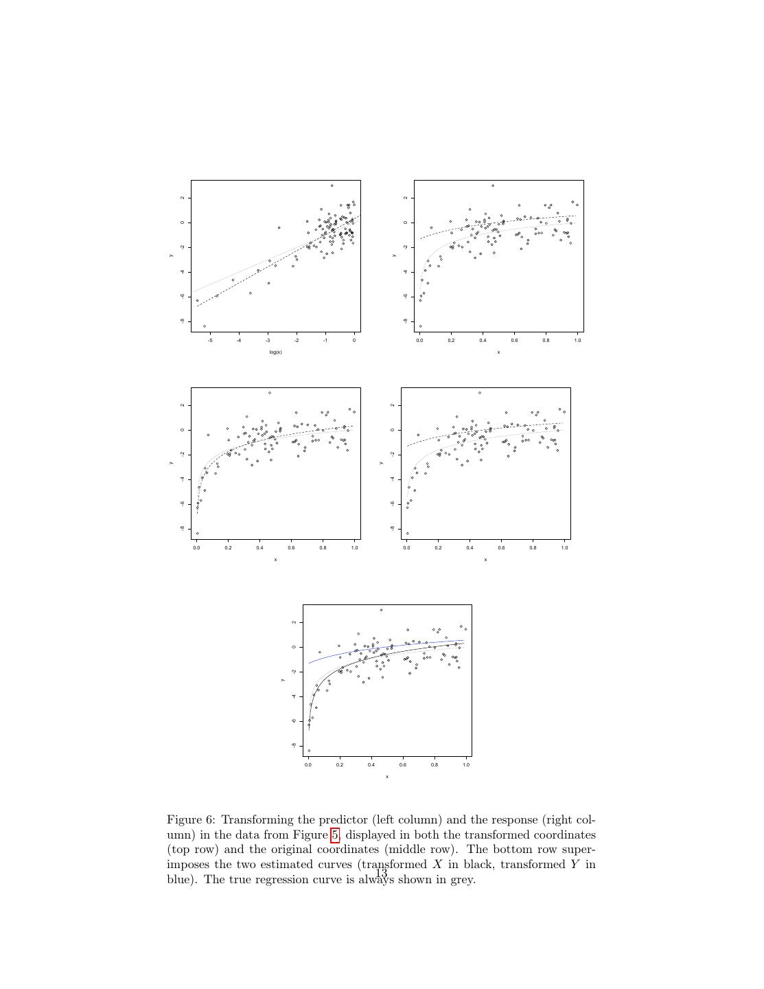
11 .one of the unanswerable questions the world is full of, as much as “what song the sirens sang, or what name Achilles took when he hid among the women”. Now, if you are willing to assume that η is a very nicely behaved Gaussian and you know its variance, then there are standard solutions to the error-in- variables problem for linear regression — ways of estimating the coefficients you’d get if you could regress Y on U . I’m not going to go over them, partly because they’re in standard textbooks, but mostly because the assumptions are hopelessly demanding. Non-parametric error-in-variable methods are an active topic of research (Carroll et al., 2009). 2.4 Transformation Let’s look at a simple non-linear example, Y |X ∼ N (log X, 1). The problem with smoothing data from this source on to a straight line is that the true regression curve isn’t very straight, E [Y |X = x] = log x. (Figure 5.) This suggests replacing the variables we have with ones where the relationship is linear, and then undoing the transformation to get back to what we actually measure and care about. We have two choices: we can transform the response Y , or the predictor X. Here transforming the response would mean regressing exp Y on X, and transforming the predictor would mean regressing Y on log X. Both kinds of transformations can be worth trying, but transforming the predictors is, in my experience, often a better bet, for three reasons. 1. Mathematically, E [f (Y )] = f (E [Y ]). A mean-squared optimal prediction of f (Y ) is not necessarily close to the transformation of an optimal predic- tion of Y . And Y is, presumably, what we really want to predict. (Here, however, it works out.) √ 2. Imagine that Y = X + log Z. There’s not going to be any particularly nice transformation of Y that makes everything linear; though there will be transformations of the features. 3. This generalizes to more complicated models with features built from mul- tiple covariates. Figure 6 shows the effect of these transformations. Here transforming the predictor does, indeed, work out more nicely; but of course I chose the example so that it does so. To expand on that last point, imagine a model like so: q r(x) = cj fj (x) (10) j=1 If we know the functions fj , we can estimate the optimal values of the coeffi- cients cj by least squares — this is a regression of the response on new features, which happen to be defined in terms of the old ones. Because the parameters are 11 

12 . 2 0 -2 y -4 -6 -8 0.0 0.2 0.4 0.6 0.8 1.0 x Figure 5: Sample of data for Y |X ∼ N (log X, 1). (Here X ∼ Unif(0, 1), and all logs are natural logs.) The true, logarithmic regression curve is shown in grey (because it’s not really observable), and the linear regression fit is shown in black. 12 

13 . 2 2 0 0 -2 -2 y y -4 -4 -6 -6 -8 -8 -5 -4 -3 -2 -1 0 0.0 0.2 0.4 0.6 0.8 1.0 log(x) x 2 2 0 0 -2 -2 y y -4 -4 -6 -6 -8 -8 0.0 0.2 0.4 0.6 0.8 1.0 0.0 0.2 0.4 0.6 0.8 1.0 x x 2 0 -2 y -4 -6 -8 0.0 0.2 0.4 0.6 0.8 1.0 x Figure 6: Transforming the predictor (left column) and the response (right col- umn) in the data from Figure 5, displayed in both the transformed coordinates (top row) and the original coordinates (middle row). The bottom row super- imposes the two estimated curves (transformed X in black, transformed Y in 13 shown in grey. blue). The true regression curve is always 

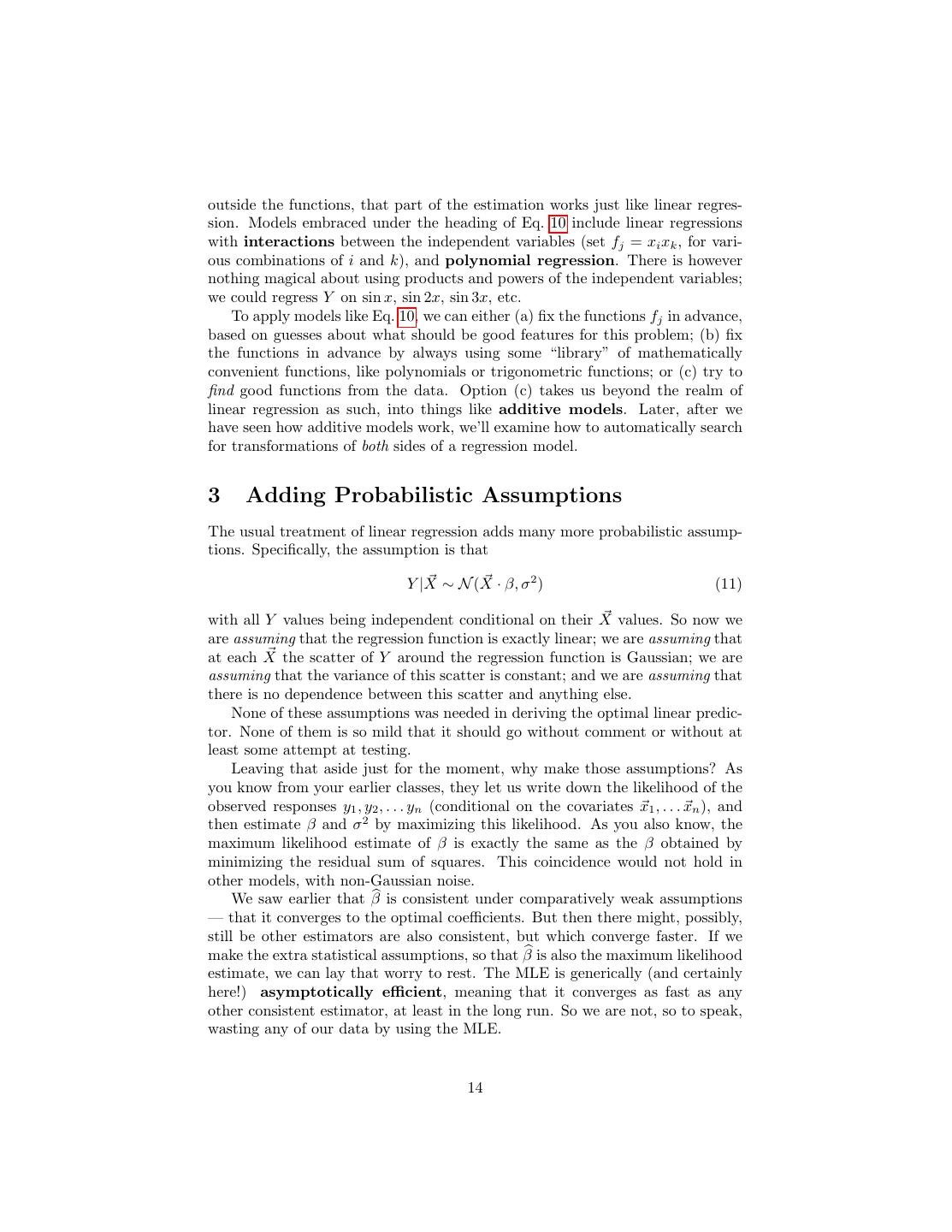
14 .outside the functions, that part of the estimation works just like linear regres- sion. Models embraced under the heading of Eq. 10 include linear regressions with interactions between the independent variables (set fj = xi xk , for vari- ous combinations of i and k), and polynomial regression. There is however nothing magical about using products and powers of the independent variables; we could regress Y on sin x, sin 2x, sin 3x, etc. To apply models like Eq. 10, we can either (a) fix the functions fj in advance, based on guesses about what should be good features for this problem; (b) fix the functions in advance by always using some “library” of mathematically convenient functions, like polynomials or trigonometric functions; or (c) try to find good functions from the data. Option (c) takes us beyond the realm of linear regression as such, into things like additive models. Later, after we have seen how additive models work, we’ll examine how to automatically search for transformations of both sides of a regression model. 3 Adding Probabilistic Assumptions The usual treatment of linear regression adds many more probabilistic assump- tions. Specifically, the assumption is that Y |X ∼ N (X · β, σ 2 ) (11) with all Y values being independent conditional on their X values. So now we are assuming that the regression function is exactly linear; we are assuming that at each X the scatter of Y around the regression function is Gaussian; we are assuming that the variance of this scatter is constant; and we are assuming that there is no dependence between this scatter and anything else. None of these assumptions was needed in deriving the optimal linear predic- tor. None of them is so mild that it should go without comment or without at least some attempt at testing. Leaving that aside just for the moment, why make those assumptions? As you know from your earlier classes, they let us write down the likelihood of the observed responses y1 , y2 , . . . yn (conditional on the covariates x1 , . . . xn ), and then estimate β and σ 2 by maximizing this likelihood. As you also know, the maximum likelihood estimate of β is exactly the same as the β obtained by minimizing the residual sum of squares. This coincidence would not hold in other models, with non-Gaussian noise. We saw earlier that β is consistent under comparatively weak assumptions — that it converges to the optimal coefficients. But then there might, possibly, still be other estimators are also consistent, but which converge faster. If we make the extra statistical assumptions, so that β is also the maximum likelihood estimate, we can lay that worry to rest. The MLE is generically (and certainly here!) asymptotically efficient, meaning that it converges as fast as any other consistent estimator, at least in the long run. So we are not, so to speak, wasting any of our data by using the MLE. 14 

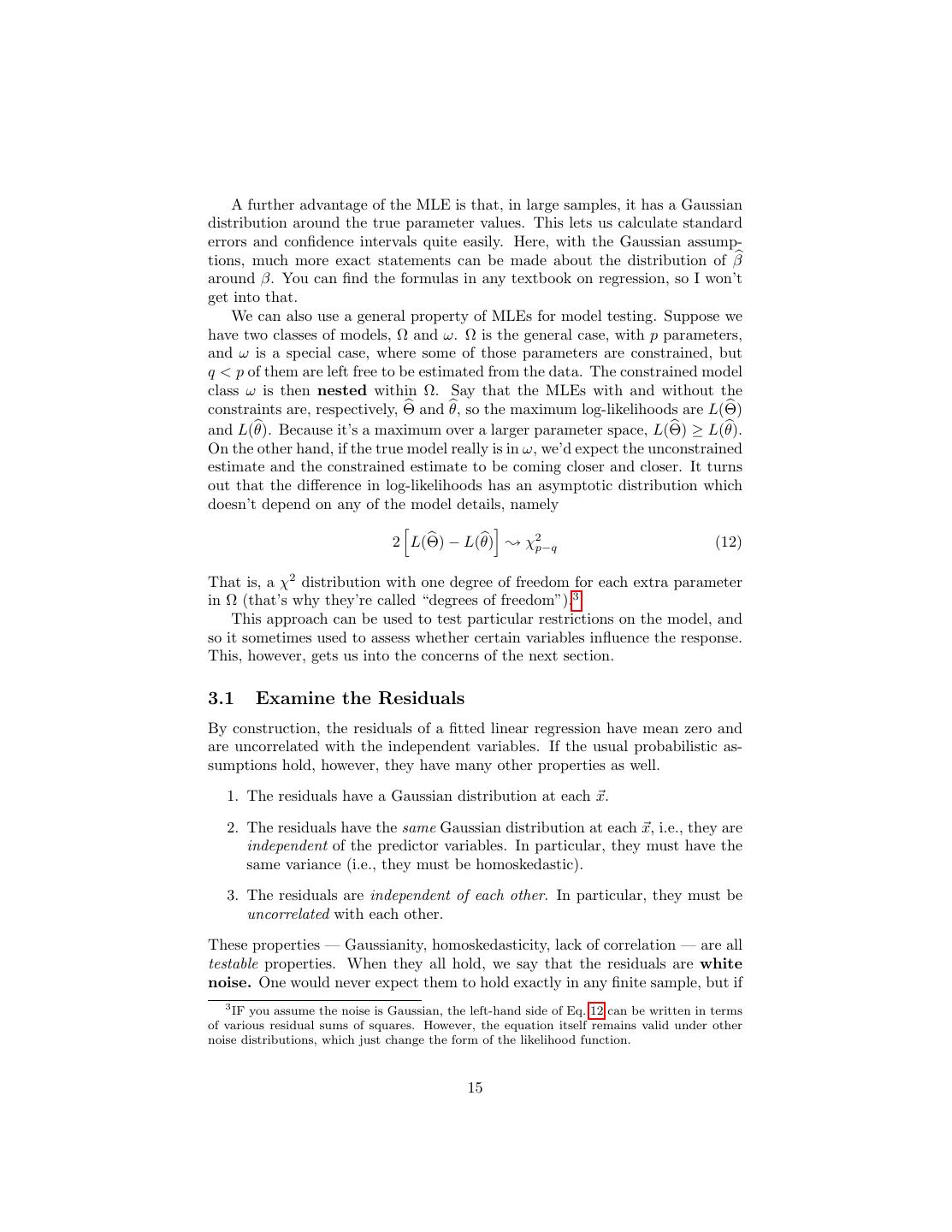
15 . A further advantage of the MLE is that, in large samples, it has a Gaussian distribution around the true parameter values. This lets us calculate standard errors and confidence intervals quite easily. Here, with the Gaussian assump- tions, much more exact statements can be made about the distribution of β around β. You can find the formulas in any textbook on regression, so I won’t get into that. We can also use a general property of MLEs for model testing. Suppose we have two classes of models, Ω and ω. Ω is the general case, with p parameters, and ω is a special case, where some of those parameters are constrained, but q < p of them are left free to be estimated from the data. The constrained model class ω is then nested within Ω. Say that the MLEs with and without the constraints are, respectively, Θ and θ, so the maximum log-likelihoods are L(Θ) and L(θ). Because it’s a maximum over a larger parameter space, L(Θ) ≥ L(θ). On the other hand, if the true model really is in ω, we’d expect the unconstrained estimate and the constrained estimate to be coming closer and closer. It turns out that the difference in log-likelihoods has an asymptotic distribution which doesn’t depend on any of the model details, namely 2 L(Θ) − L(θ) ❀ χ2p−q (12) That is, a χ2 distribution with one degree of freedom for each extra parameter in Ω (that’s why they’re called “degrees of freedom”).3 This approach can be used to test particular restrictions on the model, and so it sometimes used to assess whether certain variables influence the response. This, however, gets us into the concerns of the next section. 3.1 Examine the Residuals By construction, the residuals of a fitted linear regression have mean zero and are uncorrelated with the independent variables. If the usual probabilistic as- sumptions hold, however, they have many other properties as well. 1. The residuals have a Gaussian distribution at each x. 2. The residuals have the same Gaussian distribution at each x, i.e., they are independent of the predictor variables. In particular, they must have the same variance (i.e., they must be homoskedastic). 3. The residuals are independent of each other. In particular, they must be uncorrelated with each other. These properties — Gaussianity, homoskedasticity, lack of correlation — are all testable properties. When they all hold, we say that the residuals are white noise. One would never expect them to hold exactly in any finite sample, but if 3 IF you assume the noise is Gaussian, the left-hand side of Eq. 12 can be written in terms of various residual sums of squares. However, the equation itself remains valid under other noise distributions, which just change the form of the likelihood function. 15 

16 .you do test for them and find them strongly violated, you should be extremely suspicious of your model. These tests are much more important than checking whether the coefficients are significantly different from zero. Every time someone uses linear regression and does not test whether the residuals are white noise, an angel loses its wings. 4 Linear Regression Is Not the Philosopher’s Stone The philosopher’s stone, remember, was supposed to be able to transmute base metals (e.g., lead) into the perfect metal, gold (Eliade, 1971). Many people treat linear regression as though it had a similar ability to transmute a correlation matrix into a scientific theory. In particular, people often argue that: 1. because a variable has a non-zero regression coefficient, it must influence the response; 2. because a variable has a zero regression coefficient, it must not influence the response; 3. if the independent variables change, we can predict how much the response will change by plugging in to the regression. All of this is wrong, or at best right only under very particular circumstances. We have already seen examples where influential variables have regression coefficients of zero. We have also seen examples of situations where a variable with no influence has a non-zero coefficient (e.g., because it is correlated with an omitted variable which does have influence). If there are no nonlinearities and if there are no omitted influential variables and if the noise terms are always independent of the predictor variables, are we good? No. Remember from Equation 5 that the optimal regression coefficients depend on both the marginal distribution of the predictors and the joint dis- tribution (covariances) of the response and the predictors. There is no reason whatsoever to suppose that if we change the system, this will leave the condi- tional distribution of the response alone. A simple example may drive the point home. Suppose we surveyed all the cars in Pittsburgh, recording the maximum speed they reach over a week, and how often they are waxed and polished. I don’t think anyone doubts that there will be a positive correlation here, and in fact that there will be a positive regression coefficient, even if we add in many other variables as predictors. Let us even postulate that the relationship is linear (perhaps after a suitable transformation). Would anyone believe that waxing cars will make them go faster? Manifestly not; at best the causality goes the other way. But this is exactly how people interpret regressions in all kinds of applied fields — instead of saying waxing makes cars go faster, it might be saying that receiving targeted ads makes customers buy more, or that consuming dairy foods makes diabetes 16 

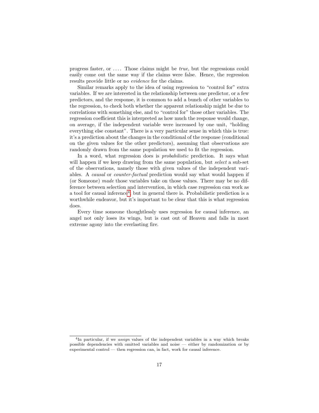
17 .progress faster, or . . . . Those claims might be true, but the regressions could easily come out the same way if the claims were false. Hence, the regression results provide little or no evidence for the claims. Similar remarks apply to the idea of using regression to “control for” extra variables. If we are interested in the relationship between one predictor, or a few predictors, and the response, it is common to add a bunch of other variables to the regression, to check both whether the apparent relationship might be due to correlations with something else, and to “control for” those other variables. The regression coefficient this is interpreted as how much the response would change, on average, if the independent variable were increased by one unit, “holding everything else constant”. There is a very particular sense in which this is true: it’s a prediction about the changes in the conditional of the response (conditional on the given values for the other predictors), assuming that observations are randomly drawn from the same population we used to fit the regression. In a word, what regression does is probabilistic prediction. It says what will happen if we keep drawing from the same population, but select a sub-set of the observations, namely those with given values of the independent vari- ables. A causal or counter-factual prediction would say what would happen if (or Someone) made those variables take on those values. There may be no dif- ference between selection and intervention, in which case regression can work as a tool for causal inference4 ; but in general there is. Probabilistic prediction is a worthwhile endeavor, but it’s important to be clear that this is what regression does. Every time someone thoughtlessly uses regression for causal inference, an angel not only loses its wings, but is cast out of Heaven and falls in most extreme agony into the everlasting fire. 4 In particular, if we assign values of the independent variables in a way which breaks possible dependencies with omitted variables and noise — either by randomization or by experimental control — then regression can, in fact, work for causal inference. 17 

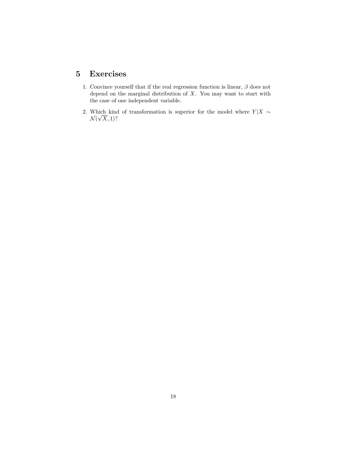
18 .5 Exercises 1. Convince yourself that if the real regression function is linear, β does not depend on the marginal distribution of X. You may want to start with the case of one independent variable. √ kind of transformation is superior for the model where Y |X ∼ 2. Which N ( X, 1)? 18 

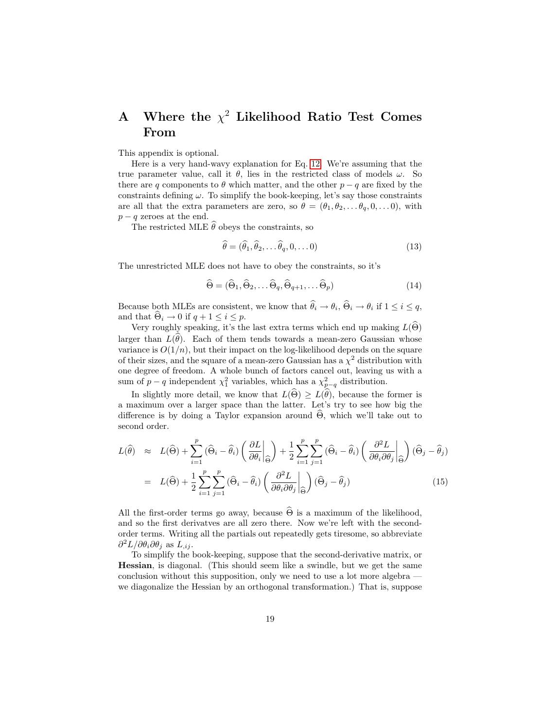
19 .A Where the χ2 Likelihood Ratio Test Comes From This appendix is optional. Here is a very hand-wavy explanation for Eq. 12. We’re assuming that the true parameter value, call it θ, lies in the restricted class of models ω. So there are q components to θ which matter, and the other p − q are fixed by the constraints defining ω. To simplify the book-keeping, let’s say those constraints are all that the extra parameters are zero, so θ = (θ1 , θ2 , . . . θq , 0, . . . 0), with p − q zeroes at the end. The restricted MLE θ obeys the constraints, so θ = (θ1 , θ2 , . . . θq , 0, . . . 0) (13) The unrestricted MLE does not have to obey the constraints, so it’s Θ = (Θ1 , Θ2 , . . . Θq , Θq+1 , . . . Θp ) (14) Because both MLEs are consistent, we know that θi → θi , Θi → θi if 1 ≤ i ≤ q, and that Θi → 0 if q + 1 ≤ i ≤ p. Very roughly speaking, it’s the last extra terms which end up making L(Θ) larger than L(θ). Each of them tends towards a mean-zero Gaussian whose variance is O(1/n), but their impact on the log-likelihood depends on the square of their sizes, and the square of a mean-zero Gaussian has a χ2 distribution with one degree of freedom. A whole bunch of factors cancel out, leaving us with a sum of p − q independent χ21 variables, which has a χ2p−q distribution. In slightly more detail, we know that L(Θ) ≥ L(θ), because the former is a maximum over a larger space than the latter. Let’s try to see how big the difference is by doing a Taylor expansion around Θ, which we’ll take out to second order. p p p ∂L 1 ∂2L L(θ) ≈ L(Θ) + (Θi − θi ) + (Θi − θi ) (Θj − θj ) i=1 ∂θi Θ 2 i=1 j=1 ∂θi ∂θj Θ p p 1 ∂2L = L(Θ) + (Θi − θi ) (Θj − θj ) (15) 2 i=1 j=1 ∂θi ∂θj Θ All the first-order terms go away, because Θ is a maximum of the likelihood, and so the first derivatves are all zero there. Now we’re left with the second- order terms. Writing all the partials out repeatedly gets tiresome, so abbreviate ∂ 2 L/∂θi ∂θj as L,ij . To simplify the book-keeping, suppose that the second-derivative matrix, or Hessian, is diagonal. (This should seem like a swindle, but we get the same conclusion without this supposition, only we need to use a lot more algebra — we diagonalize the Hessian by an orthogonal transformation.) That is, suppose 19 

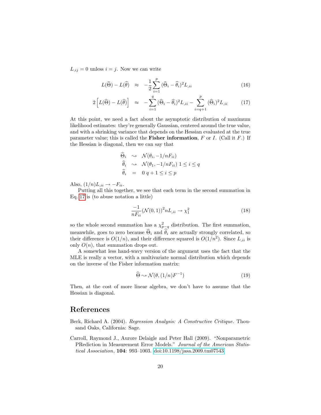
20 .L,ij = 0 unless i = j. Now we can write p 1 L(Θ) − L(θ) ≈ − (Θi − θi )2 L,ii (16) 2 i=1 q p 2 L(Θ) − L(θ) ≈ − (Θi − θi )2 L,ii − (Θi )2 L,ii (17) i=1 i=q+1 At this point, we need a fact about the asymptotic distribution of maximum likelihood estimates: they’re generally Gaussian, centered around the true value, and with a shrinking variance that depends on the Hessian evaluated at the true parameter value; this is called the Fisher information, F or I. (Call it F .) If the Hessian is diagonal, then we can say that Θi ❀ N (θi , −1/nFii ) θi ❀ N (θ1 , −1/nFii ) 1 ≤ i ≤ q θi = 0 q+1≤i≤p Also, (1/n)L,ii → −Fii . Putting all this together, we see that each term in the second summation in Eq. 17 is (to abuse notation a little) −1 2 (N (0, 1)) nL,ii → χ21 (18) nFii so the whole second summation has a χ2p−q distribution. The first summation, meanwhile, goes to zero because Θi and θi are actually strongly correlated, so their difference is O(1/n), and their difference squared is O(1/n2 ). Since L,ii is only O(n), that summation drops out. A somewhat less hand-wavy version of the argument uses the fact that the MLE is really a vector, with a multivariate normal distribution which depends on the inverse of the Fisher information matrix: Θ ❀ N (θ, (1/n)F −1 ) (19) Then, at the cost of more linear algebra, we don’t have to assume that the Hessian is diagonal. References Berk, Richard A. (2004). Regression Analysis: A Constructive Critique. Thou- sand Oaks, California: Sage. Carroll, Raymond J., Aurore Delaigle and Peter Hall (2009). “Nonparametric PRediction in Measurement Error Models.” Journal of the American Statis- tical Association, 104: 993–1003. doi:10.1198/jasa.2009.tm07543. 20 

21 .Eliade, Mircea (1971). The Forge and the Crucible: The Origin and Structure of Alchemy. New York: Harper and Row. Faraway, Julian (2004). Linear Models with R. Boca Raton, Florida: Chapman and Hall/CRC Press. 21