Support Vector Machines

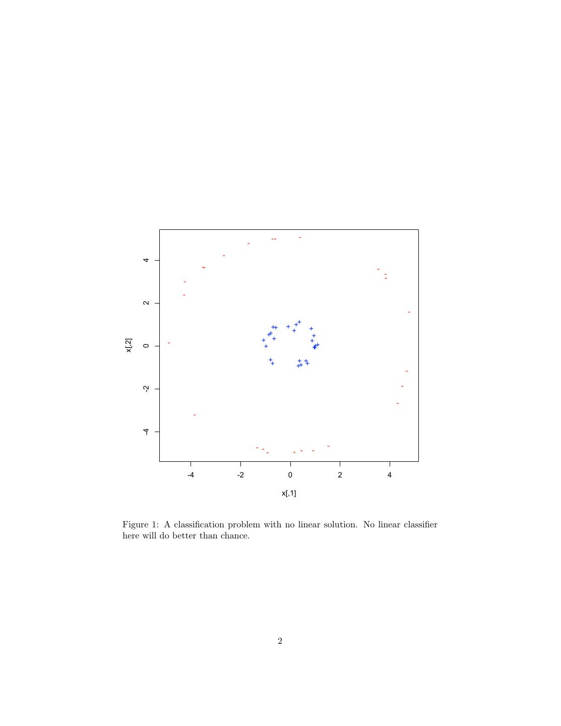
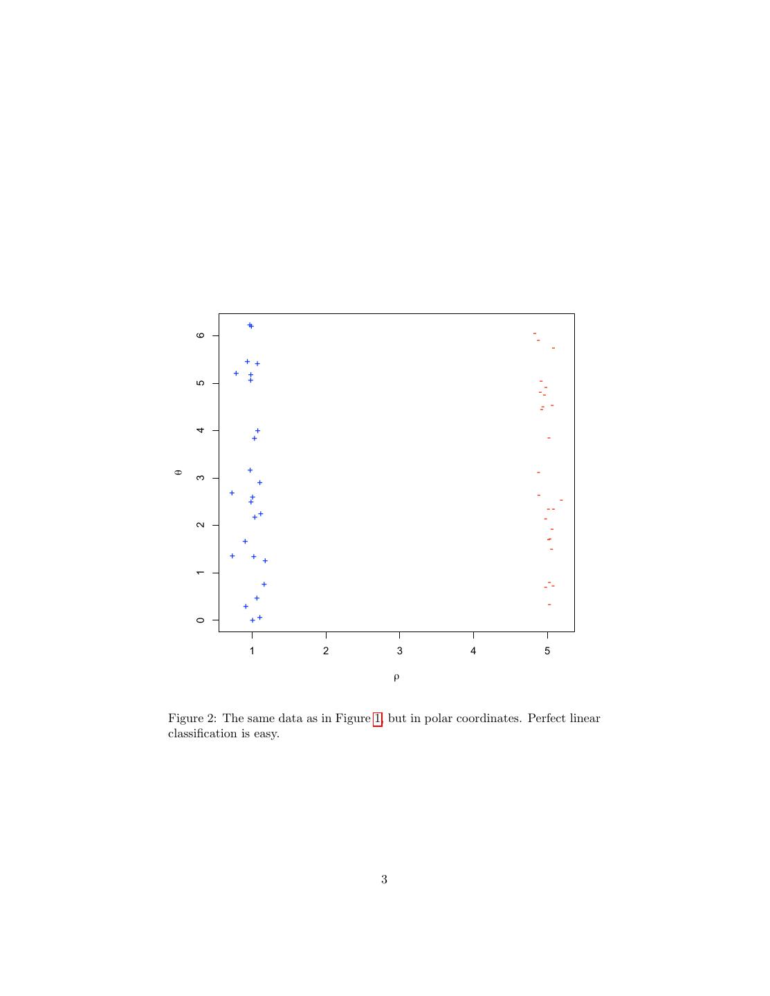
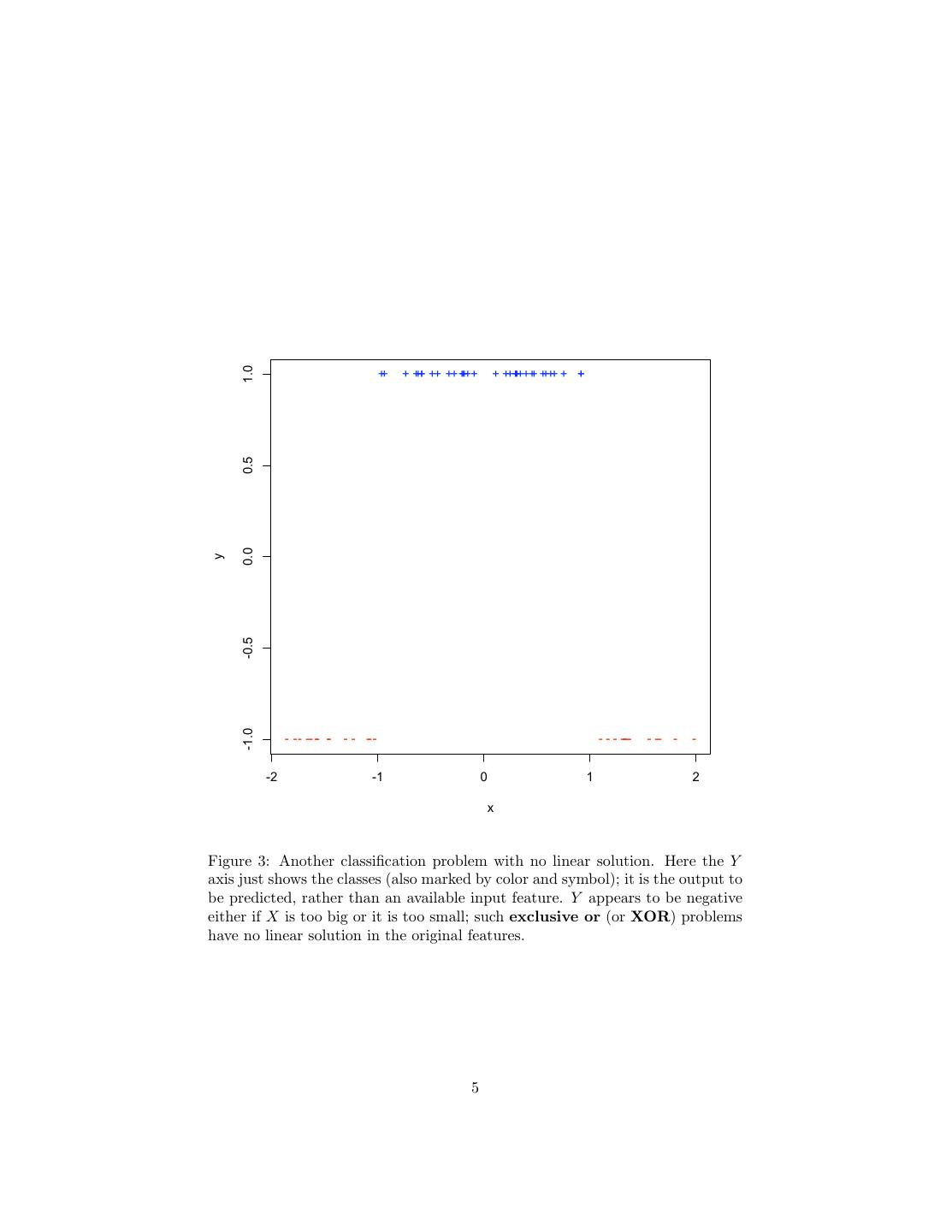
1 . Support Vector Machines 36-350, Data Mining, Fall 2009 20 November 2009 Contents 1 Why We Want to Use Many Nonlinear Features, But Don’t Actually Want to Calculate Them 1 2 Dual Representation and Support Vectors 7 3 The Kernel Trick 7 4 Margin Bounds 10 5 The Support Vector Machine 12 5.1 Maximum Margin SVMs . . . . . . . . . . . . . . . . . . . . . . . 13 5.2 Soft Margin Maximization . . . . . . . . . . . . . . . . . . . . . . 13 6 R 14 1 Why We Want to Use Many Nonlinear Fea- tures, But Don’t Actually Want to Calculate Them Neural networks work by creating new features in the hidden layer. This, as has been repeatedly emphasized, is one of the keys to successful machine learning: finding the right transformations of the input makes the problem easy in the new features. For example, looking at the data in Figure 1 in Cartesian (rectangular) coordinates, the problem of classifying points as + or − is moderately hard — there is in fact no linear classifier which does better than chance at this. On the other hand, if I have the wit to guess the new features ρ = x21 + x22 and θ = arctan x2 /x1 , then I get a dead-simple classification problem, where perfect linear separation is easy (Figure 2). In this example, we kept the number of features the same, but it’s often useful to create more new features than we had originally. Figure 3 shows a one-dimensional classification problem which has no linear solution: the class is negative if x is below some threshold or above another threshold, but not both. 1 

2 . -- - - - 4 -- - -- - - 2 - + ++ + + + + ++ + + + + x[,2] - + +++ 0 ++ ++ ++ + - - -2 - - -4 - - - - - - - -4 -2 0 2 4 x[,1] Figure 1: A classification problem with no linear solution. No linear classifier here will do better than chance. 2 

3 . ++ - 6 - - ++ + + + - 5 - -- -- - + 4 + - + - θ 3 + + - ++ - -- ++ - 2 - + -- - + + + 1 + - -- + + - ++ 0 1 2 3 4 5 ρ Figure 2: The same data as in Figure 1, but in polar coordinates. Perfect linear classification is easy. 3 

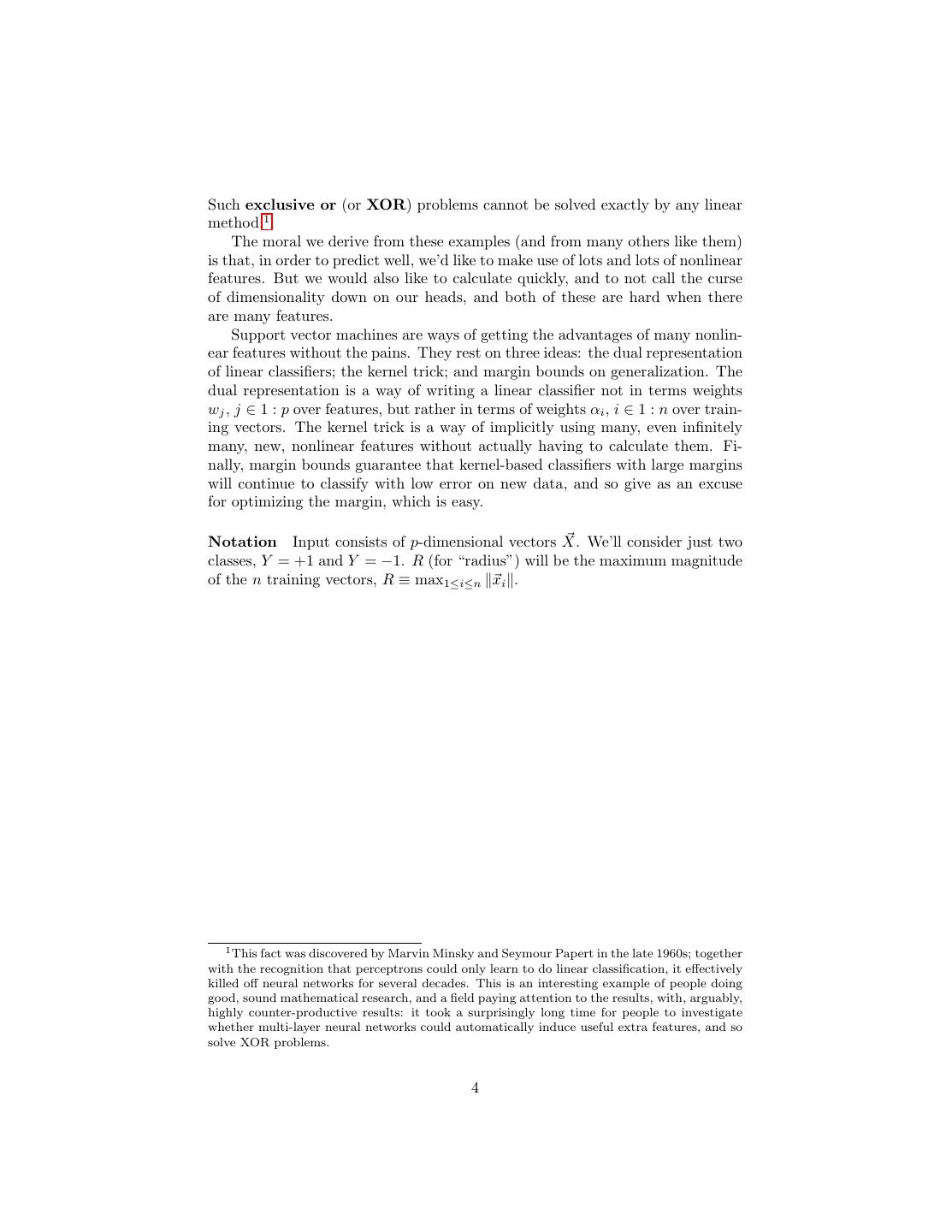
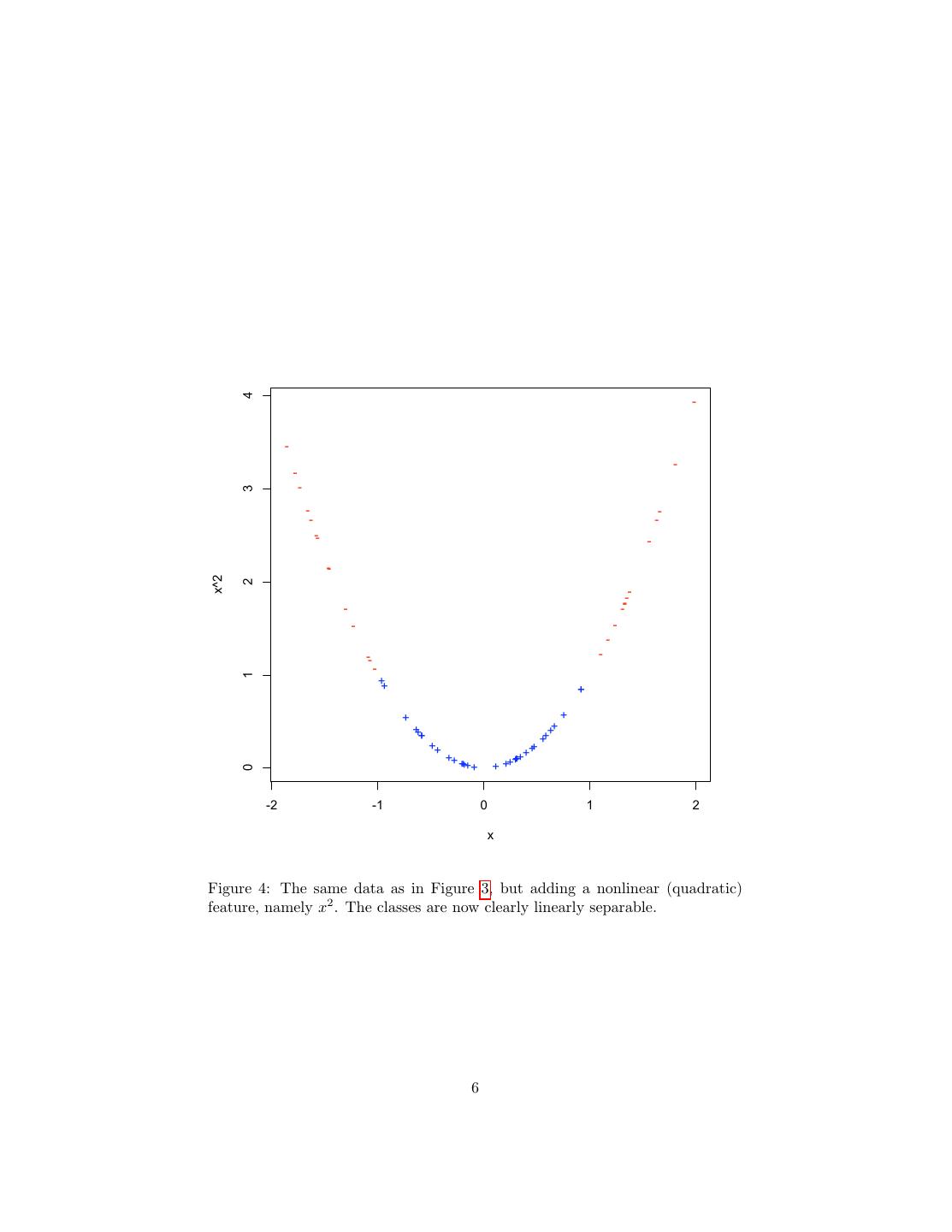
4 .Such exclusive or (or XOR) problems cannot be solved exactly by any linear method.1 The moral we derive from these examples (and from many others like them) is that, in order to predict well, we’d like to make use of lots and lots of nonlinear features. But we would also like to calculate quickly, and to not call the curse of dimensionality down on our heads, and both of these are hard when there are many features. Support vector machines are ways of getting the advantages of many nonlin- ear features without the pains. They rest on three ideas: the dual representation of linear classifiers; the kernel trick; and margin bounds on generalization. The dual representation is a way of writing a linear classifier not in terms weights wj , j ∈ 1 : p over features, but rather in terms of weights αi , i ∈ 1 : n over train- ing vectors. The kernel trick is a way of implicitly using many, even infinitely many, new, nonlinear features without actually having to calculate them. Fi- nally, margin bounds guarantee that kernel-based classifiers with large margins will continue to classify with low error on new data, and so give as an excuse for optimizing the margin, which is easy. Notation Input consists of p-dimensional vectors X. We’ll consider just two classes, Y = +1 and Y = −1. R (for “radius”) will be the maximum magnitude of the n training vectors, R ≡ max1≤i≤n xi . 1 This fact was discovered by Marvin Minsky and Seymour Papert in the late 1960s; together with the recognition that perceptrons could only learn to do linear classification, it effectively killed off neural networks for several decades. This is an interesting example of people doing good, sound mathematical research, and a field paying attention to the results, with, arguably, highly counter-productive results: it took a surprisingly long time for people to investigate whether multi-layer neural networks could automatically induce useful extra features, and so solve XOR problems. 4 

5 . 1.0 ++ + +++ ++ ++++++ + +++++++ + ++++ + + 0.5 0.0 y -0.5 -1.0 - - - -- - - - - -- - - - - ---- - -- - - -2 -1 0 1 2 x Figure 3: Another classification problem with no linear solution. Here the Y axis just shows the classes (also marked by color and symbol); it is the output to be predicted, rather than an available input feature. Y appears to be negative either if X is too big or it is too small; such exclusive or (or XOR) problems have no linear solution in the original features. 5 

6 . 4 - - - - - 3 - - - - -- - - x^2 2 -- - -- - - - -- - - 1 ++ + + + +++ ++ ++ ++ +++ +++ +++ +++ + ++ 0 -2 -1 0 1 2 x Figure 4: The same data as in Figure 3, but adding a nonlinear (quadratic) feature, namely x2 . The classes are now clearly linearly separable. 6 

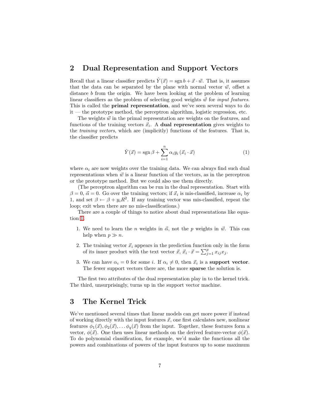
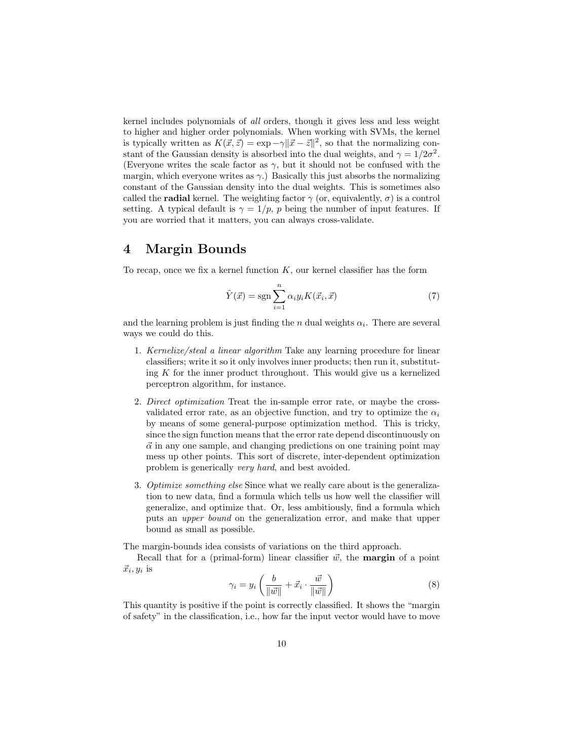
7 .2 Dual Representation and Support Vectors Recall that a linear classifier predicts Yˆ (x) = sgn b + x · w. That is, it assumes that the data can be separated by the plane with normal vector w, offset a distance b from the origin. We have been looking at the problem of learning linear classifiers as the problem of selecting good weights w for input features. This is called the primal representation, and we’ve seen several ways to do it — the prototype method, the perceptron algorithm, logistic regression, etc. The weights w in the primal representation are weights on the features, and functions of the training vectors xi . A dual representation gives weights to the training vectors, which are (implicitly) functions of the features. That is, the classifier predicts n Yˆ (x) = sgn β + αi yi (xi · x) (1) i=1 where αi are now weights over the training data. We can always find such dual representations when w is a linear function of the vectors, as in the perceptron or the prototype method. But we could also use them directly. (The perceptron algorithm can be run in the dual representation. Start with β = 0, α = 0. Go over the training vectors; if xi is mis-classified, increase αi by 1, and set β ← β + yi R2 . If any training vector was mis-classified, repeat the loop; exit when there are no mis-classifications.) There are a couple of things to notice about dual representations like equa- tion 1. 1. We need to learn the n weights in α, not the p weights in w. This can help when p n. 2. The training vector xi appears in the prediction function only in the form p of its inner product with the text vector x, xi · x = j=1 xij xj . 3. We can have αi = 0 for some i. If αi = 0, then xi is a support vector. The fewer support vectors there are, the more sparse the solution is. The first two attributes of the dual representation play in to the kernel trick. The third, unsurprisingly, turns up in the support vector machine. 3 The Kernel Trick We’ve mentioned several times that linear models can get more power if instead of working directly with the input features x, one first calculates new, nonlinear features φ1 (x), φ2 (x), . . . φq (x) from the input. Together, these features form a vector, φ(x). One then uses linear methods on the derived feature-vector φ(x). To do polynomial classification, for example, we’d make the functions all the powers and combinations of powers of the input features up to some maximum 7 

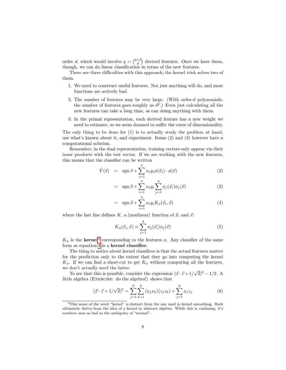
8 .order d, which would involve q = p+d d derived features. Once we have them, though, we can do linear classification in terms of the new features. There are three difficulties with this approach; the kernel trick solves two of them. 1. We need to construct useful features. Not just anything will do, and most functions are actively bad. 2. The number of features may be very large. (With order-d polynomials, the number of features goes roughly as dp .) Even just calculating all the new features can take a long time, as can doing anything with them. 3. In the primal representation, each derived feature has a new weight we need to estimate, so we seem doomed to suffer the curse of dimensionality. The only thing to be done for (1) is to actually study the problem at hand, use what’s known about it, and experiment. Items (2) and (3) however have a computational solution. Remember, in the dual representation, training vectors only appear via their inner products with the test vector. If we are working with the new features, this means that the classifier can be written n Yˆ (x) = sgn β + αi yi φ(xi ) · φ(x) (2) i=1 n q = sgn β + αi yi φj (xi )φj (x) (3) i=1 j=1 n = sgn β + αi yi Kφ (xi , x) (4) i=1 where the last line defines K, a (nonlinear) function of xi and x: q Kφ (xi , x) ≡ φj (xi )φj (x) (5) j=1 Kφ is the kernel2 corresponding to the features φ. Any classifier of the same form as equation 4 is a kernel classifier. The thing to notice about kernel classifiers is that the actual features matter for the prediction only to the extent that they go into computing the kernel Kφ . If we can find a short-cut to get Kφ without computing all the features, we don’t actually need the latter. √ To see that this is possible, consider the expression (x · z + 1/ 2)2 − 1/2. A little algebra (Exercise: do the algebra!) shows that p p p √ (x · z + 1/ 2)2 = (xj xk )(zj zk ) + xj zj (6) j=1 k=1 j=1 2 This sense of the word “kernel” is distinct from the one used in kernel smoothing. Both ultimately derive from the idea of a kernel in abstract algebra. While this is confusing, it’s nowhere near as bad as the ambiguity of “normal”. 8 

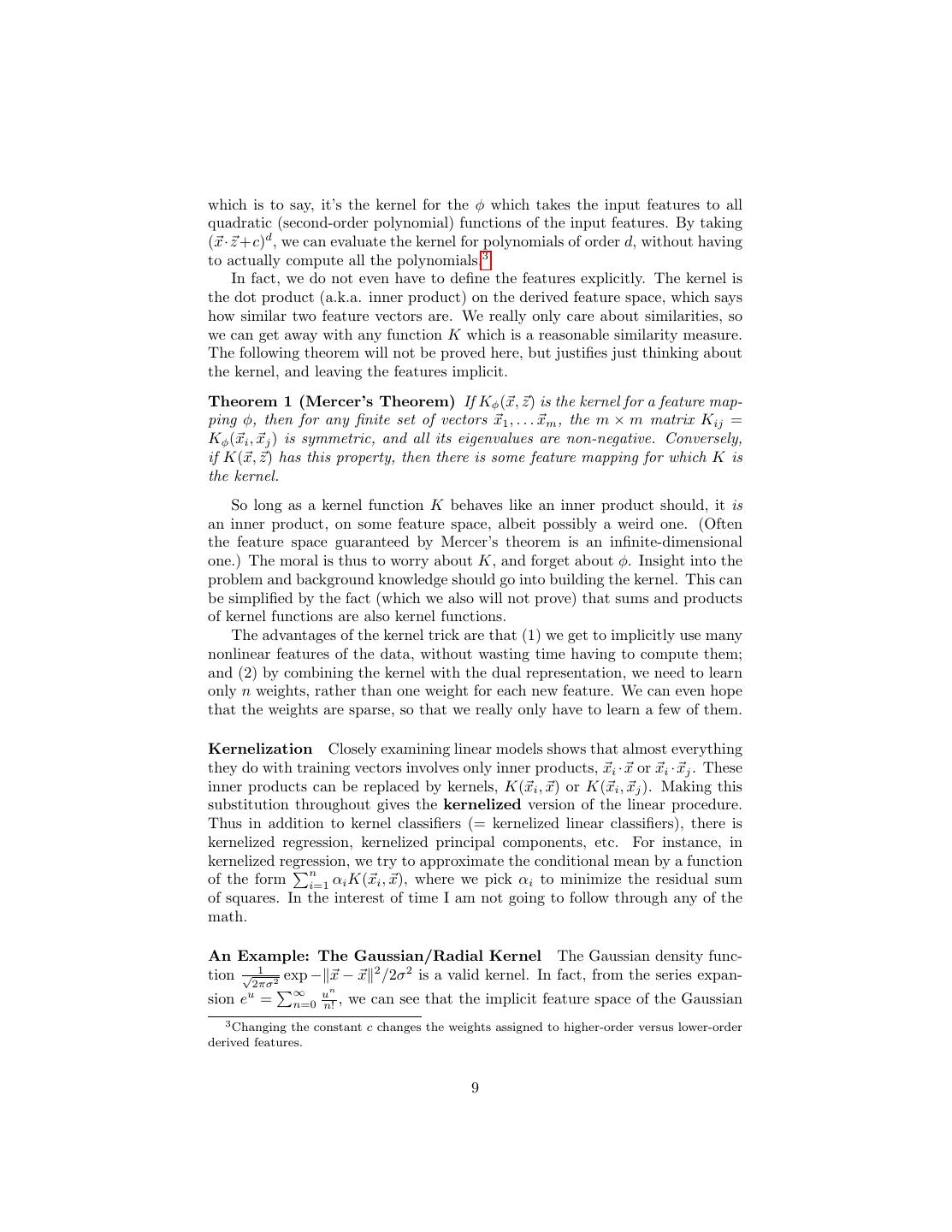
9 .which is to say, it’s the kernel for the φ which takes the input features to all quadratic (second-order polynomial) functions of the input features. By taking (x·z +c)d , we can evaluate the kernel for polynomials of order d, without having to actually compute all the polynomials.3 In fact, we do not even have to define the features explicitly. The kernel is the dot product (a.k.a. inner product) on the derived feature space, which says how similar two feature vectors are. We really only care about similarities, so we can get away with any function K which is a reasonable similarity measure. The following theorem will not be proved here, but justifies just thinking about the kernel, and leaving the features implicit. Theorem 1 (Mercer’s Theorem) If Kφ (x, z) is the kernel for a feature map- ping φ, then for any finite set of vectors x1 , . . . xm , the m × m matrix Kij = Kφ (xi , xj ) is symmetric, and all its eigenvalues are non-negative. Conversely, if K(x, z) has this property, then there is some feature mapping for which K is the kernel. So long as a kernel function K behaves like an inner product should, it is an inner product, on some feature space, albeit possibly a weird one. (Often the feature space guaranteed by Mercer’s theorem is an infinite-dimensional one.) The moral is thus to worry about K, and forget about φ. Insight into the problem and background knowledge should go into building the kernel. This can be simplified by the fact (which we also will not prove) that sums and products of kernel functions are also kernel functions. The advantages of the kernel trick are that (1) we get to implicitly use many nonlinear features of the data, without wasting time having to compute them; and (2) by combining the kernel with the dual representation, we need to learn only n weights, rather than one weight for each new feature. We can even hope that the weights are sparse, so that we really only have to learn a few of them. Kernelization Closely examining linear models shows that almost everything they do with training vectors involves only inner products, xi ·x or xi ·xj . These inner products can be replaced by kernels, K(xi , x) or K(xi , xj ). Making this substitution throughout gives the kernelized version of the linear procedure. Thus in addition to kernel classifiers (= kernelized linear classifiers), there is kernelized regression, kernelized principal components, etc. For instance, in kernelized regression, we try to approximate the conditional mean by a function n of the form i=1 αi K(xi , x), where we pick αi to minimize the residual sum of squares. In the interest of time I am not going to follow through any of the math. An Example: The Gaussian/Radial Kernel The Gaussian density func- 1 tion √2πσ 2 exp − x − x 2 /2σ 2 is a valid kernel. In fact, from the series expan- ∞ un sion eu = n=0 n! , we can see that the implicit feature space of the Gaussian 3 Changing the constant c changes the weights assigned to higher-order versus lower-order derived features. 9 

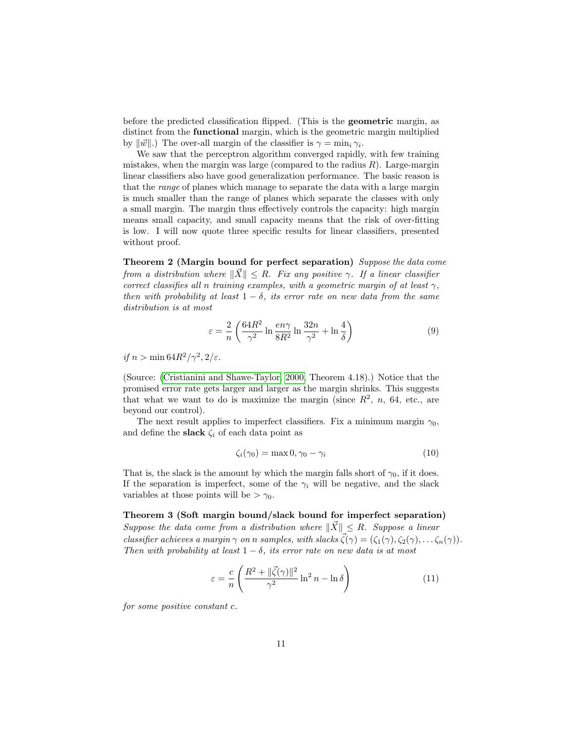
10 .kernel includes polynomials of all orders, though it gives less and less weight to higher and higher order polynomials. When working with SVMs, the kernel is typically written as K(x, z) = exp −γ x − z 2 , so that the normalizing con- stant of the Gaussian density is absorbed into the dual weights, and γ = 1/2σ 2 . (Everyone writes the scale factor as γ, but it should not be confused with the margin, which everyone writes as γ.) Basically this just absorbs the normalizing constant of the Gaussian density into the dual weights. This is sometimes also called the radial kernel. The weighting factor γ (or, equivalently, σ) is a control setting. A typical default is γ = 1/p, p being the number of input features. If you are worried that it matters, you can always cross-validate. 4 Margin Bounds To recap, once we fix a kernel function K, our kernel classifier has the form n Yˆ (x) = sgn αi yi K(xi , x) (7) i=1 and the learning problem is just finding the n dual weights αi . There are several ways we could do this. 1. Kernelize/steal a linear algorithm Take any learning procedure for linear classifiers; write it so it only involves inner products; then run it, substitut- ing K for the inner product throughout. This would give us a kernelized perceptron algorithm, for instance. 2. Direct optimization Treat the in-sample error rate, or maybe the cross- validated error rate, as an objective function, and try to optimize the αi by means of some general-purpose optimization method. This is tricky, since the sign function means that the error rate depend discontinuously on α in any one sample, and changing predictions on one training point may mess up other points. This sort of discrete, inter-dependent optimization problem is generically very hard, and best avoided. 3. Optimize something else Since what we really care about is the generaliza- tion to new data, find a formula which tells us how well the classifier will generalize, and optimize that. Or, less ambitiously, find a formula which puts an upper bound on the generalization error, and make that upper bound as small as possible. The margin-bounds idea consists of variations on the third approach. Recall that for a (primal-form) linear classifier w, the margin of a point xi , yi is b w γi = yi + xi · (8) w w This quantity is positive if the point is correctly classified. It shows the “margin of safety” in the classification, i.e., how far the input vector would have to move 10 

11 .before the predicted classification flipped. (This is the geometric margin, as distinct from the functional margin, which is the geometric margin multiplied by w .) The over-all margin of the classifier is γ = mini γi . We saw that the perceptron algorithm converged rapidly, with few training mistakes, when the margin was large (compared to the radius R). Large-margin linear classifiers also have good generalization performance. The basic reason is that the range of planes which manage to separate the data with a large margin is much smaller than the range of planes which separate the classes with only a small margin. The margin thus effectively controls the capacity: high margin means small capacity, and small capacity means that the risk of over-fitting is low. I will now quote three specific results for linear classifiers, presented without proof. Theorem 2 (Margin bound for perfect separation) Suppose the data come from a distribution where X ≤ R. Fix any positive γ. If a linear classifier correct classifies all n training examples, with a geometric margin of at least γ, then with probability at least 1 − δ, its error rate on new data from the same distribution is at most 2 64R2 enγ 32n 4 ε= ln ln 2 + ln (9) n γ2 8R2 γ δ if n > min 64R2 /γ 2 , 2/ε. (Source: (Cristianini and Shawe-Taylor, 2000, Theorem 4.18).) Notice that the promised error rate gets larger and larger as the margin shrinks. This suggests that what we want to do is maximize the margin (since R2 , n, 64, etc., are beyond our control). The next result applies to imperfect classifiers. Fix a minimum margin γ0 , and define the slack ζi of each data point as ζi (γ0 ) = max 0, γ0 − γi (10) That is, the slack is the amount by which the margin falls short of γ0 , if it does. If the separation is imperfect, some of the γi will be negative, and the slack variables at those points will be > γ0 . Theorem 3 (Soft margin bound/slack bound for imperfect separation) Suppose the data come from a distribution where X ≤ R. Suppose a linear classifier achieves a margin γ on n samples, with slacks ζ(γ) = (ζ1 (γ), ζ2 (γ), . . . ζn (γ)). Then with probability at least 1 − δ, its error rate on new data is at most c R2 + ζ(γ) 2 ε= ln2 n − ln δ (11) n γ2 for some positive constant c. 11 

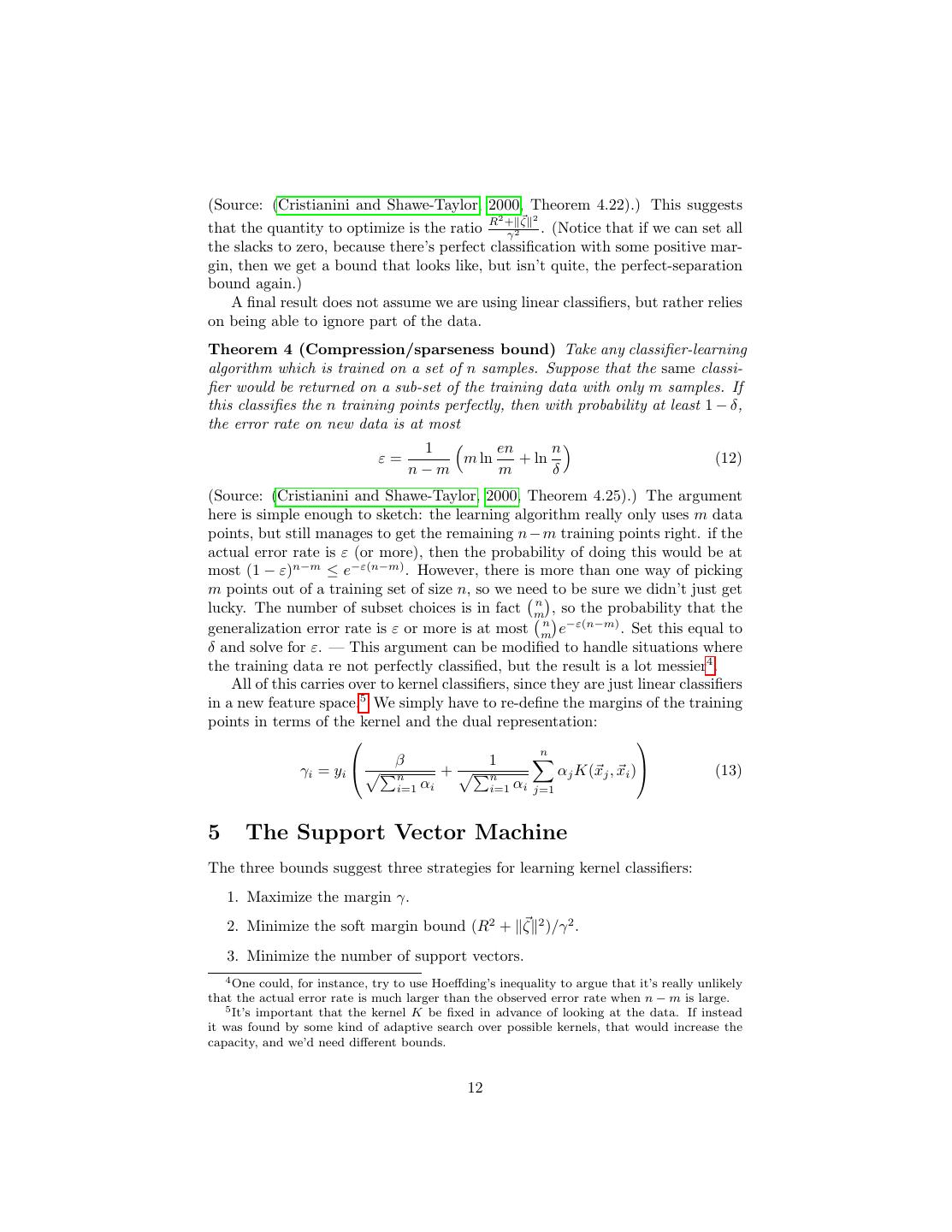
12 .(Source: (Cristianini and Shawe-Taylor, 2000, Theorem 4.22).) This suggests 2 2 that the quantity to optimize is the ratio R +γ 2ζ . (Notice that if we can set all the slacks to zero, because there’s perfect classification with some positive mar- gin, then we get a bound that looks like, but isn’t quite, the perfect-separation bound again.) A final result does not assume we are using linear classifiers, but rather relies on being able to ignore part of the data. Theorem 4 (Compression/sparseness bound) Take any classifier-learning algorithm which is trained on a set of n samples. Suppose that the same classi- fier would be returned on a sub-set of the training data with only m samples. If this classifies the n training points perfectly, then with probability at least 1 − δ, the error rate on new data is at most 1 en n ε= m ln + ln (12) n−m m δ (Source: (Cristianini and Shawe-Taylor, 2000, Theorem 4.25).) The argument here is simple enough to sketch: the learning algorithm really only uses m data points, but still manages to get the remaining n − m training points right. if the actual error rate is ε (or more), then the probability of doing this would be at most (1 − ε)n−m ≤ e−ε(n−m) . However, there is more than one way of picking m points out of a training set of size n, so we need to be sure we didn’t just get n lucky. The number of subset choices is in fact m , so the probability that the n −ε(n−m) generalization error rate is ε or more is at most m e . Set this equal to δ and solve for ε. — This argument can be modified to handle situations where the training data re not perfectly classified, but the result is a lot messier4 . All of this carries over to kernel classifiers, since they are just linear classifiers in a new feature space.5 We simply have to re-define the margins of the training points in terms of the kernel and the dual representation:   n β 1 γi = yi  n + n αj K(xj , xi ) (13) i=1 αi i=1 αi j=1 5 The Support Vector Machine The three bounds suggest three strategies for learning kernel classifiers: 1. Maximize the margin γ. 2. Minimize the soft margin bound (R2 + ζ 2 )/γ 2 . 3. Minimize the number of support vectors. 4 One could, for instance, try to use Hoeffding’s inequality to argue that it’s really unlikely that the actual error rate is much larger than the observed error rate when n − m is large. 5 It’s important that the kernel K be fixed in advance of looking at the data. If instead it was found by some kind of adaptive search over possible kernels, that would increase the capacity, and we’d need different bounds. 12 

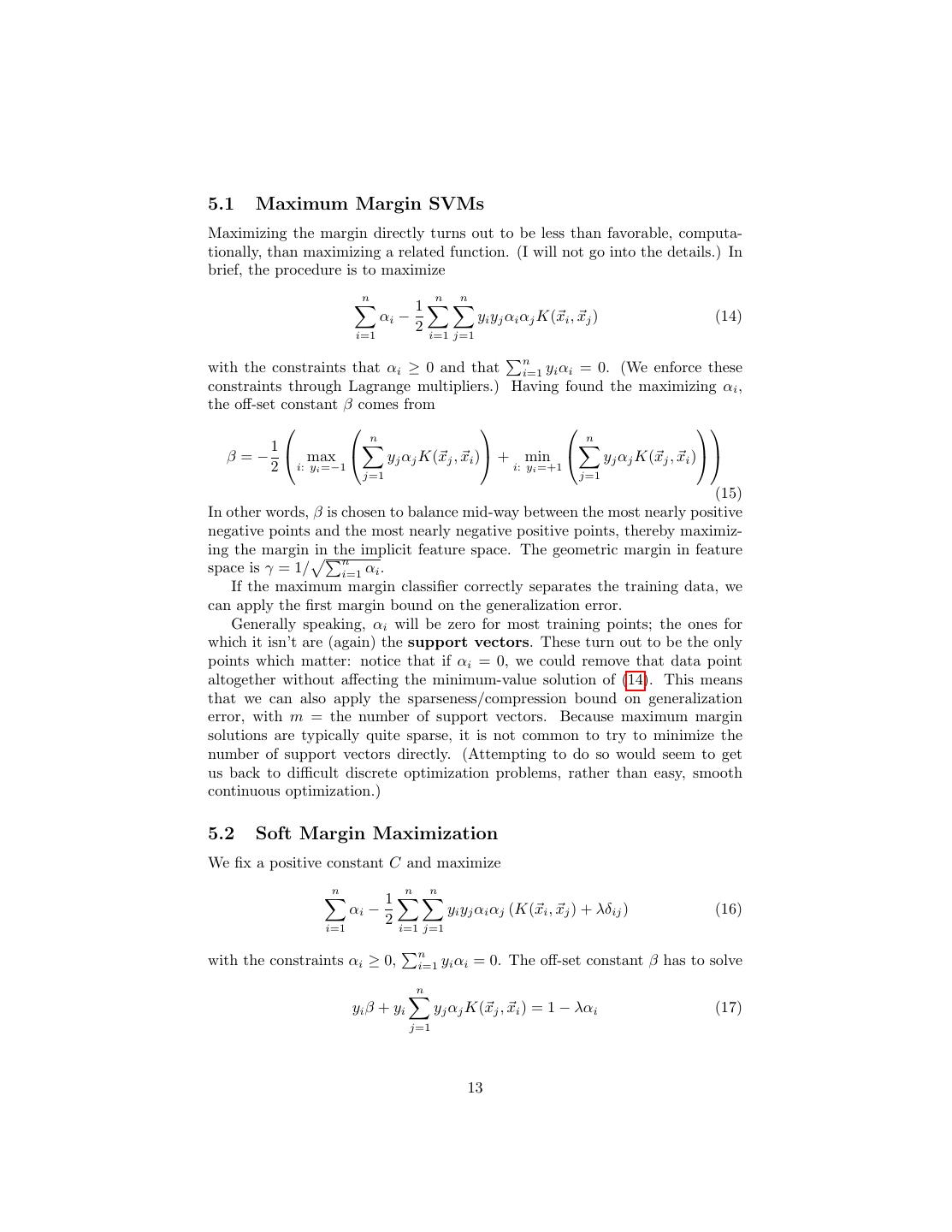
13 .5.1 Maximum Margin SVMs Maximizing the margin directly turns out to be less than favorable, computa- tionally, than maximizing a related function. (I will not go into the details.) In brief, the procedure is to maximize n n n 1 αi − yi yj αi αj K(xi , xj ) (14) i=1 2 i=1 j=1 n with the constraints that αi ≥ 0 and that i=1 yi αi = 0. (We enforce these constraints through Lagrange multipliers.) Having found the maximizing αi , the off-set constant β comes from      n n 1 β=− max  yj αj K(xj , xi ) + min  yj αj K(xj , xi ) 2 i: yi =−1 j=1 i: yi =+1 j=1 (15) In other words, β is chosen to balance mid-way between the most nearly positive negative points and the most nearly negative positive points, thereby maximiz- ing the margin in the implicit feature space. The geometric margin in feature n space is γ = 1/ i=1 αi . If the maximum margin classifier correctly separates the training data, we can apply the first margin bound on the generalization error. Generally speaking, αi will be zero for most training points; the ones for which it isn’t are (again) the support vectors. These turn out to be the only points which matter: notice that if αi = 0, we could remove that data point altogether without affecting the minimum-value solution of (14). This means that we can also apply the sparseness/compression bound on generalization error, with m = the number of support vectors. Because maximum margin solutions are typically quite sparse, it is not common to try to minimize the number of support vectors directly. (Attempting to do so would seem to get us back to difficult discrete optimization problems, rather than easy, smooth continuous optimization.) 5.2 Soft Margin Maximization We fix a positive constant C and maximize n n n 1 αi − yi yj αi αj (K(xi , xj ) + λδij ) (16) i=1 2 i=1 j=1 n with the constraints αi ≥ 0, i=1 yi αi = 0. The off-set constant β has to solve n yi β + yi yj αj K(xj , xi ) = 1 − λαi (17) j=1 13 

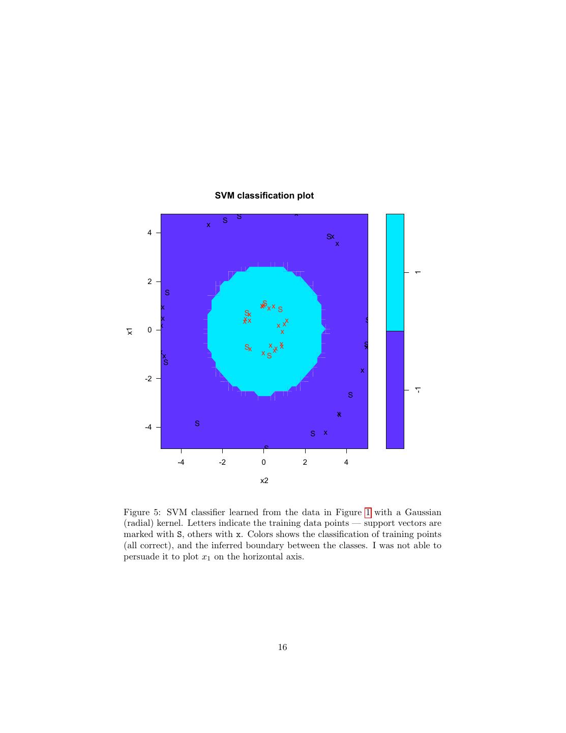
14 .for each i where αi = 0. Pick one of them and solve for β: n 1 − λαi β= − yj αj K(xj , xi ) (18) yi j=1 2 The geometric margin is γ = 1/ i=1 nαi − λ α , and the slacks are ζi = λαi . The constant λ here is a tuning parameter, basically controlling the trade-off between wanting a large margin and wanting small slacks. Typically, it would be chosen by cross-validation. 6 R There are several packages which can implement SVMs. The oddly-named e1071 library has an svm function which will take lm-style formulas, and can do either classification or regression with several different kernels. The svmpath library will actually fit SVMs over a whole range of λ values simultaneously; but you have to pick a particular λ for prediction. (It also doesn’t take a formula argument or allow you to do regression.) For instance, the data for Figure 1 live in a frame called, imaginatively, rings, with columns named x1 (real numbers), x2 (real numbers) and y (cate- gorical values, i.e. “factors” in R). To fit an SVM to this data, use rings.svm = svm(y ~ ., data=rings) The formula y . means “include every variable in the frame other than the response in the model”.6 Since the response variable is a factor, the svm function defaults to doing classification — if I’d made y have the numerical values +1 and −1, svm would default to regression, and I’d have to give an extra type argument to the function to tell it to classify. (See help(svm).) Other defaults include the kernel (here the Gaussian/radial kernel) and the value of λ (the svm function uses a cost argument = 1/λ, defaulting to 1). Because this is such a simple problem, the defaults work perfectly. > sum(predict(rings.svm) != rings$y) [1] 0 We can plot the classifier as well (Figure 5). plot(rings.svm,data=my.frame,color.palette=topo.colors, svSymbol="S",dataSymbol="x") The plot function for svm objects requires a data set, and with more than two input features it would need extra argument saying which variables to plot, and what values to impose on the others. (I don’t like the default color or symbol 6 If you know regular expressions, remember that . matches any character. If you don’t know regular expressions, don’t worry about it. 14 

15 .choices, so I changed them.) In the plot, you’ll see an S for the data points which are support vectors, and an x for the others. You can also see the boundary between the two classes. Note that the support vectors in each class are closer to the boundary than the other vectors in that class, as they should be. Further Reading The best starting book on support vector machines, which I’ve ripped off drawn on heavily is Cristianini and Shawe-Taylor (2000). A more thorough account of SVMs and related methods can be had in Herbrich (2002). SVMs were invented by Vapnik and collaborators, and are, so to speak, the poster-children for the value of statistical learning theory in machine learning and data mining; Vapnik (2000) is strongly recommended, but remember that you’re reading the pronouncements of an opinionated and irascible genius. References Cristianini, Nello and John Shawe-Taylor (2000). An Introduction to Support Vector Machines: And Other Kernel-Based Learning Methods. Cambridge, England: Cambridge University Press. Herbrich, Ralf (2002). Learning Kernel Classifiers: Theory and Algorithms. Cambridge, Massachusetts: MIT Press. Vapnik, Vladimir N. (2000). The Nature of Statistical Learning Theory. Berlin: Springer-Verlag, 2nd edn. 15 

16 . SVM classification plot S x x S 4 Sx x 1 2 S x xxSx x Sx S x xxx x S x xx 0 x x1 Sx x x xx S x x x x Sx S x -2 -1 S xx -4 S S x S -4 -2 0 2 4 x2 Figure 5: SVM classifier learned from the data in Figure 1 with a Gaussian (radial) kernel. Letters indicate the training data points — support vectors are marked with S, others with x. Colors shows the classification of training points (all correct), and the inferred boundary between the classes. I was not able to persuade it to plot x1 on the horizontal axis. 16