Smoothing Methods in Regression

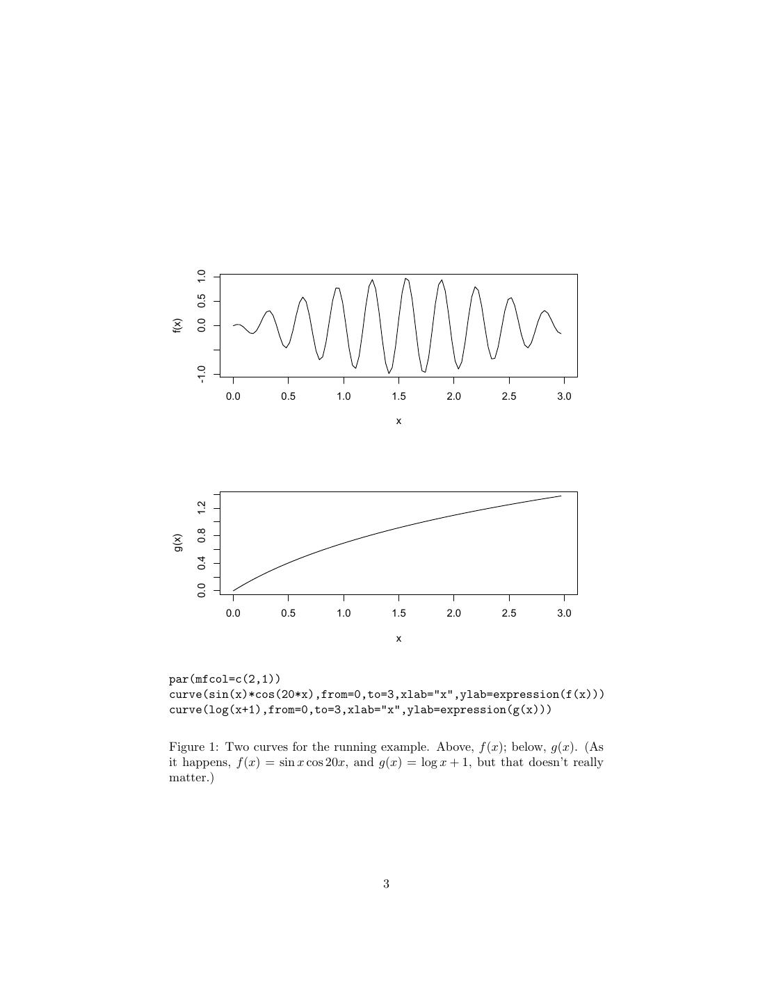
1 . Using Nonparametric Smoothing: Adaptation and Testing Parametric Models 36-350, Data Mining 30 October 2009 Contents 1 How Much Smoothing? Adapting to Unknown Roughness 1 2 Testing Functional Forms 14 2.1 Examples of Testing a Parametric Model . . . . . . . . . . . . . . 16 2.2 Why Use Parametric Models At All? . . . . . . . . . . . . . . . . 20 We are still talking about regression, i.e., a supervised learning problem. Recall the basic kind of smoothing we are interested in: we have a response variable Y , some input variables which we bind up into a vector X, and a collection of data values, (x1 , y1 ), (x2 , y2 ), . . . xn , yn ). By “smoothing”, I mean that predictions are going to be weighted averages of the observed responses in the training data: n r(x) = yi w(x, xi , h) (1) i=1 Most smoothing methods have a control setting, which here I write h, that determines how much smoothing we do. With k nearest neighbors, for instance, the weights are 1/k if xi is one of the k-nearest points to x, and w = 0 otherwise, so large k means that each prediction is an average over many training points. Similarly with kernel regression, where the degree of smoothing is controlled by the bandwidth h. Why do we want to do this? How do we pick how much smoothing to do? 1 How Much Smoothing? Adapting to Unknown Roughness Consider Figure 1, which graphs two functions, f and g. Both are “smooth” functions in the qualitative, mathematical sense (C ∞ : they’re not only con- tinuous, their derivatives exist and are continuous to all orders). We could Taylor expand both functions to approximate their values anywhere, just from 1 

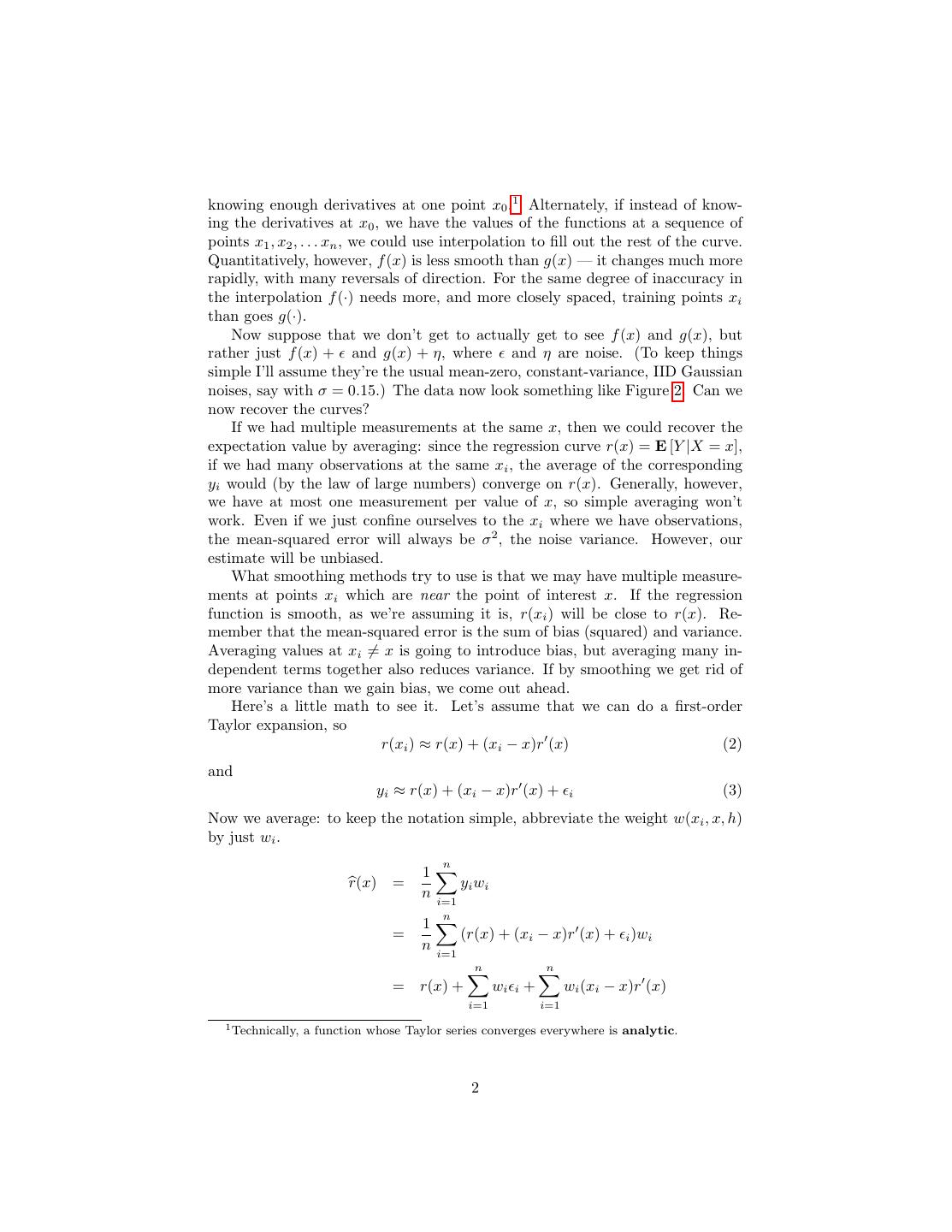
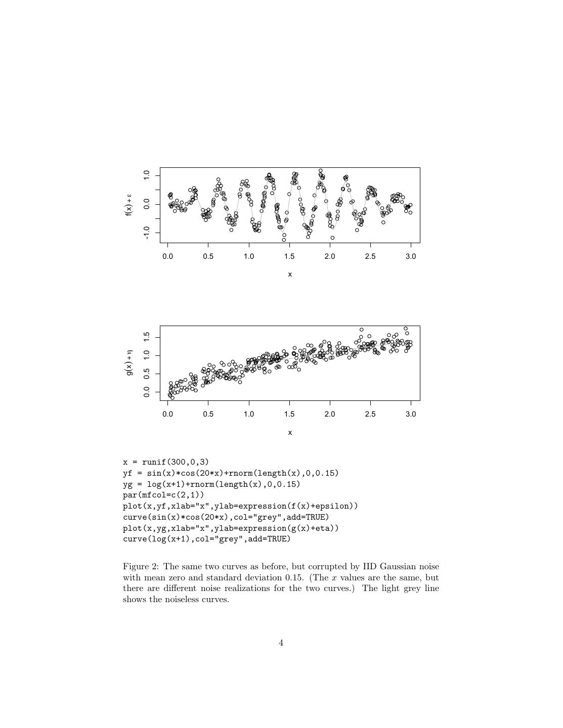
2 .knowing enough derivatives at one point x0 .1 Alternately, if instead of know- ing the derivatives at x0 , we have the values of the functions at a sequence of points x1 , x2 , . . . xn , we could use interpolation to fill out the rest of the curve. Quantitatively, however, f (x) is less smooth than g(x) — it changes much more rapidly, with many reversals of direction. For the same degree of inaccuracy in the interpolation f (·) needs more, and more closely spaced, training points xi than goes g(·). Now suppose that we don’t get to actually get to see f (x) and g(x), but rather just f (x) + and g(x) + η, where and η are noise. (To keep things simple I’ll assume they’re the usual mean-zero, constant-variance, IID Gaussian noises, say with σ = 0.15.) The data now look something like Figure 2. Can we now recover the curves? If we had multiple measurements at the same x, then we could recover the expectation value by averaging: since the regression curve r(x) = E [Y |X = x], if we had many observations at the same xi , the average of the corresponding yi would (by the law of large numbers) converge on r(x). Generally, however, we have at most one measurement per value of x, so simple averaging won’t work. Even if we just confine ourselves to the xi where we have observations, the mean-squared error will always be σ 2 , the noise variance. However, our estimate will be unbiased. What smoothing methods try to use is that we may have multiple measure- ments at points xi which are near the point of interest x. If the regression function is smooth, as we’re assuming it is, r(xi ) will be close to r(x). Re- member that the mean-squared error is the sum of bias (squared) and variance. Averaging values at xi = x is going to introduce bias, but averaging many in- dependent terms together also reduces variance. If by smoothing we get rid of more variance than we gain bias, we come out ahead. Here’s a little math to see it. Let’s assume that we can do a first-order Taylor expansion, so r(xi ) ≈ r(x) + (xi − x)r (x) (2) and yi ≈ r(x) + (xi − x)r (x) + i (3) Now we average: to keep the notation simple, abbreviate the weight w(xi , x, h) by just wi . n 1 r(x) = yi wi n i=1 n 1 = (r(x) + (xi − x)r (x) + i )wi n i=1 n n = r(x) + wi i + wi (xi − x)r (x) i=1 i=1 1 Technically, a function whose Taylor series converges everywhere is analytic. 2 

3 . 0.0 0.5 1.0 f(x) -1.0 0.0 0.5 1.0 1.5 2.0 2.5 3.0 x 1.2 0.8 g(x) 0.4 0.0 0.0 0.5 1.0 1.5 2.0 2.5 3.0 x par(mfcol=c(2,1)) curve(sin(x)*cos(20*x),from=0,to=3,xlab="x",ylab=expression(f(x))) curve(log(x+1),from=0,to=3,xlab="x",ylab=expression(g(x))) Figure 1: Two curves for the running example. Above, f (x); below, g(x). (As it happens, f (x) = sin x cos 20x, and g(x) = log x + 1, but that doesn’t really matter.) 3 

4 . 1.0 f(x) + ε 0.0 -1.0 0.0 0.5 1.0 1.5 2.0 2.5 3.0 x 1.5 g(x) + η 1.0 0.5 0.0 0.0 0.5 1.0 1.5 2.0 2.5 3.0 x x = runif(300,0,3) yf = sin(x)*cos(20*x)+rnorm(length(x),0,0.15) yg = log(x+1)+rnorm(length(x),0,0.15) par(mfcol=c(2,1)) plot(x,yf,xlab="x",ylab=expression(f(x)+epsilon)) curve(sin(x)*cos(20*x),col="grey",add=TRUE) plot(x,yg,xlab="x",ylab=expression(g(x)+eta)) curve(log(x+1),col="grey",add=TRUE) Figure 2: The same two curves as before, but corrupted by IID Gaussian noise with mean zero and standard deviation 0.15. (The x values are the same, but there are different noise realizations for the two curves.) The light grey line shows the noiseless curves. 4 

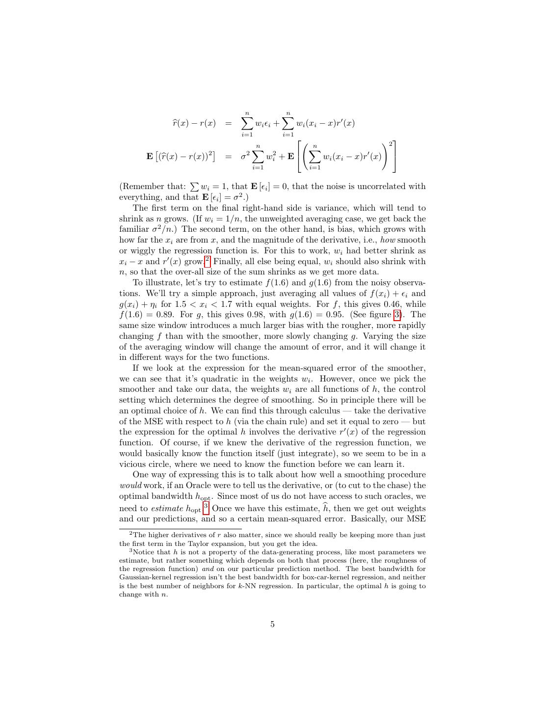
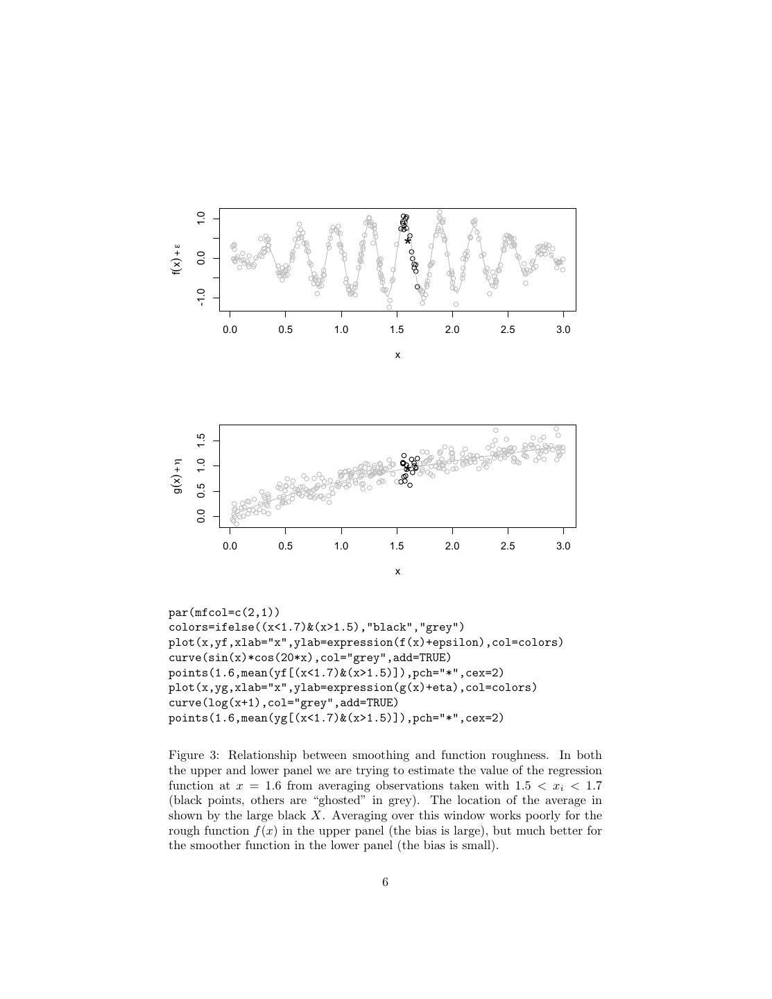
5 . n n r(x) − r(x) = wi i + wi (xi − x)r (x) i=1 i=1   n n 2 E (r(x) − r(x))2 = σ2 wi2 + E  wi (xi − x)r (x)  i=1 i=1 (Remember that: wi = 1, that E [ i ] = 0, that the noise is uncorrelated with everything, and that E [ i ] = σ 2 .) The first term on the final right-hand side is variance, which will tend to shrink as n grows. (If wi = 1/n, the unweighted averaging case, we get back the familiar σ 2 /n.) The second term, on the other hand, is bias, which grows with how far the xi are from x, and the magnitude of the derivative, i.e., how smooth or wiggly the regression function is. For this to work, wi had better shrink as xi − x and r (x) grow.2 Finally, all else being equal, wi should also shrink with n, so that the over-all size of the sum shrinks as we get more data. To illustrate, let’s try to estimate f (1.6) and g(1.6) from the noisy observa- tions. We’ll try a simple approach, just averaging all values of f (xi ) + i and g(xi ) + ηi for 1.5 < xi < 1.7 with equal weights. For f , this gives 0.46, while f (1.6) = 0.89. For g, this gives 0.98, with g(1.6) = 0.95. (See figure 3). The same size window introduces a much larger bias with the rougher, more rapidly changing f than with the smoother, more slowly changing g. Varying the size of the averaging window will change the amount of error, and it will change it in different ways for the two functions. If we look at the expression for the mean-squared error of the smoother, we can see that it’s quadratic in the weights wi . However, once we pick the smoother and take our data, the weights wi are all functions of h, the control setting which determines the degree of smoothing. So in principle there will be an optimal choice of h. We can find this through calculus — take the derivative of the MSE with respect to h (via the chain rule) and set it equal to zero — but the expression for the optimal h involves the derivative r (x) of the regression function. Of course, if we knew the derivative of the regression function, we would basically know the function itself (just integrate), so we seem to be in a vicious circle, where we need to know the function before we can learn it. One way of expressing this is to talk about how well a smoothing procedure would work, if an Oracle were to tell us the derivative, or (to cut to the chase) the optimal bandwidth hopt . Since most of us do not have access to such oracles, we need to estimate hopt .3 Once we have this estimate, h, then we get out weights and our predictions, and so a certain mean-squared error. Basically, our MSE 2 The higher derivatives of r also matter, since we should really be keeping more than just the first term in the Taylor expansion, but you get the idea. 3 Notice that h is not a property of the data-generating process, like most parameters we estimate, but rather something which depends on both that process (here, the roughness of the regression function) and on our particular prediction method. The best bandwidth for Gaussian-kernel regression isn’t the best bandwidth for box-car-kernel regression, and neither is the best number of neighbors for k-NN regression. In particular, the optimal h is going to change with n. 5 

6 . 1.0 * f(x) + ε 0.0 -1.0 0.0 0.5 1.0 1.5 2.0 2.5 3.0 x 1.5 g(x) + η 1.0 * 0.5 0.0 0.0 0.5 1.0 1.5 2.0 2.5 3.0 x par(mfcol=c(2,1)) colors=ifelse((x<1.7)&(x>1.5),"black","grey") plot(x,yf,xlab="x",ylab=expression(f(x)+epsilon),col=colors) curve(sin(x)*cos(20*x),col="grey",add=TRUE) points(1.6,mean(yf[(x<1.7)&(x>1.5)]),pch="*",cex=2) plot(x,yg,xlab="x",ylab=expression(g(x)+eta),col=colors) curve(log(x+1),col="grey",add=TRUE) points(1.6,mean(yg[(x<1.7)&(x>1.5)]),pch="*",cex=2) Figure 3: Relationship between smoothing and function roughness. In both the upper and lower panel we are trying to estimate the value of the regression function at x = 1.6 from averaging observations taken with 1.5 < xi < 1.7 (black points, others are “ghosted” in grey). The location of the average in shown by the large black X. Averaging over this window works poorly for the rough function f (x) in the upper panel (the bias is large), but much better for the smoother function in the lower panel (the bias is small). 6 

7 . 1.0 0.8 Absolute value of error 0.6 0.4 0.2 0.0 0.0 0.2 0.4 0.6 0.8 1.0 Radius of averaging window loc_ave_err <- function(h,y,y0) {abs(y0-mean(y[(1.6-h < x) & (1.6+h>x)]))} yf0=sin(1.6)*cos(20*1.6) yg0=log(1+1.6) f.LAE = sapply(0:100/100,loc_ave_err,y=yf,y0=yf0) g.LAE = sapply(0:100/100,loc_ave_err,y=yg,y0=yg0) plot(0:100/100,f.LAE,xlab="Radius of averaging window", ylab="Absolute value of error",type="l") lines(0:100/100,g.LAE,lty=2) abline(h=0.15,col="grey") Figure 4: Estimating f (1.6) and g(1.6) from averaging observed values at 1.6 − h < x < 1.6 + h, for different radii h. Solid line: error of estimates of f (1.6); dashed line: error of estimates of g(1.6); grey line: σ, the standard deviation of the noise. 7 

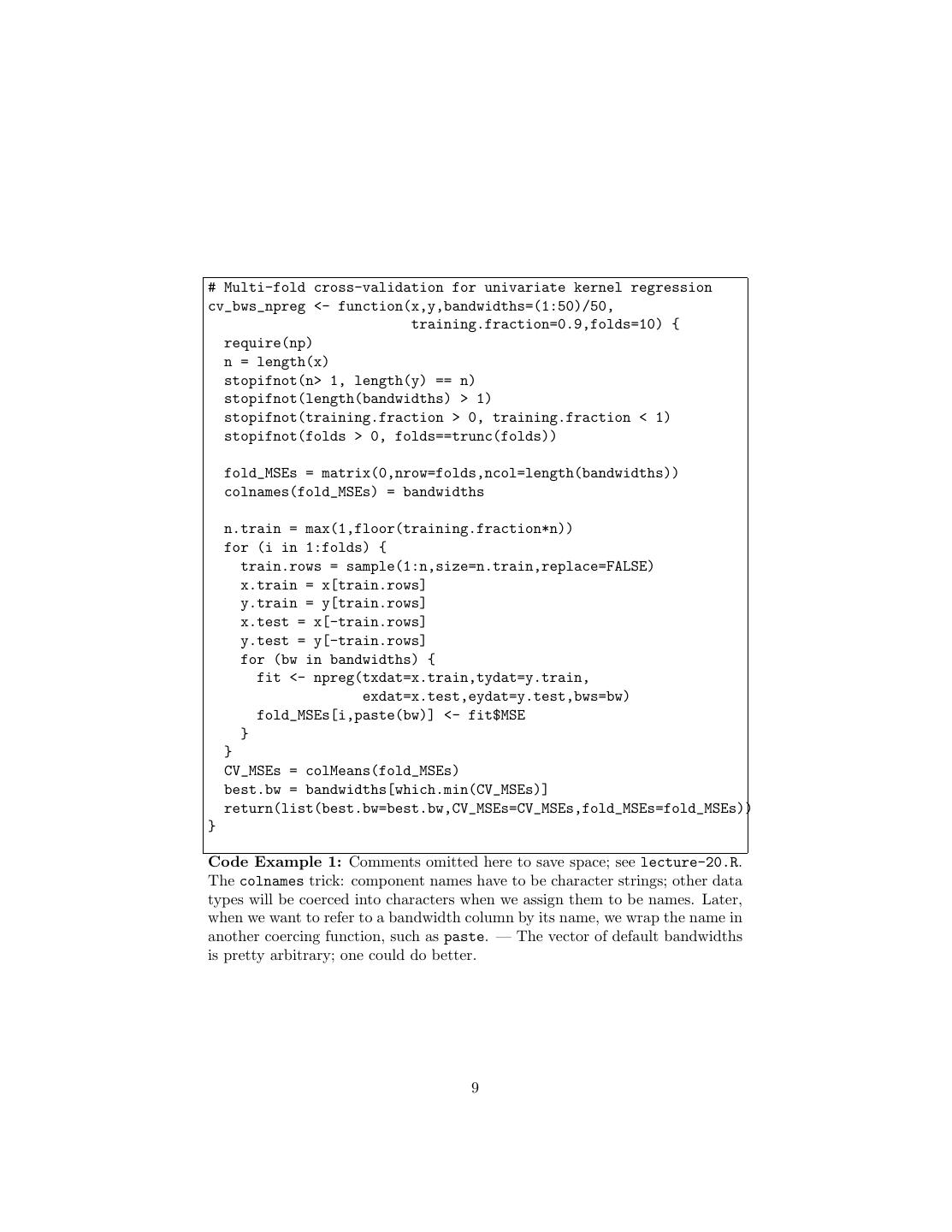
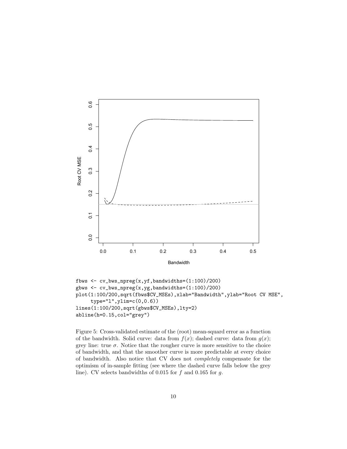
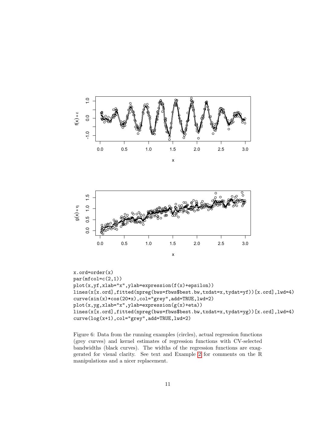
8 .will be the Oracle’s MSE, plus an extra term which depends on how far h is to hopt , and how sensitive the smoother is to the choice of bandwidth. What would be really nice would be an adaptive procedure, one where our actual MSE, using h, approaches the Oracle’s MSE, which it gets from hopt . This would mean that, in effect, we are figuring out how rough the underlying regression function is, and so how much smoothing to do, rather than having to guess or be told. An adaptive procedure, if we can find one, is a partial4 substitute for prior knowledge. The most straight-forward way to pick a bandwidth, and one which generally manages to be adaptive, is in fact cross-validation; k-fold CV is usually some- what better than leave-one-out, but the latter often works acceptably too. The random-division CV would work in the usual way, going over a grid of possible bandwidths. Here is how it would work with the input variable being in the vector x (one dimensional) and the response in the vector y (one dimensional), and using the npreg function from the np library (Hayfield and Racine, 2008).5 The return value has three parts. The first is the actual best bandwidth. The second is a vector which gives the cross-validated mean-squared mean- squared errors of all the different bandwidths in the vector bandwidths. The third component is an array which gives the MSE for each bandwidth on each fold. It can be useful to know things like whether the difference between the CV score of the best bandwidth and the runner-up is bigger than their fold-to-fold variability. Figure 5 plots the CV estimate of the (root) mean-squared error versus bandwidth for our two curves. Figure 6 shows the data, the actual regression functions and the estimated curves with the CV-selected bandwidths. The R manipulations in Figure 6 were work-arounds for the inflexibility of the plot method supplied in the np package. It’s nicer to encapsulate that sort of thing into our own functions (Example 2). Another thing we’ll want to encapsulate in a single function is selecting the bandwidth by CV and then actually fitting the model with that bandwidth. 4 Only partial, because we’d always do better if the Oracle would just tell us hopt . 5 The np package actually has a function, npregbw, which automatically selects bandwidths through a sophisticated combination of leave-one-out cross-validation and optimization tech- niques. It tends to be very slow. 8 

9 .# Multi-fold cross-validation for univariate kernel regression cv_bws_npreg <- function(x,y,bandwidths=(1:50)/50, training.fraction=0.9,folds=10) { require(np) n = length(x) stopifnot(n> 1, length(y) == n) stopifnot(length(bandwidths) > 1) stopifnot(training.fraction > 0, training.fraction < 1) stopifnot(folds > 0, folds==trunc(folds)) fold_MSEs = matrix(0,nrow=folds,ncol=length(bandwidths)) colnames(fold_MSEs) = bandwidths n.train = max(1,floor(training.fraction*n)) for (i in 1:folds) { train.rows = sample(1:n,size=n.train,replace=FALSE) x.train = x[train.rows] y.train = y[train.rows] x.test = x[-train.rows] y.test = y[-train.rows] for (bw in bandwidths) { fit <- npreg(txdat=x.train,tydat=y.train, exdat=x.test,eydat=y.test,bws=bw) fold_MSEs[i,paste(bw)] <- fit$MSE } } CV_MSEs = colMeans(fold_MSEs) best.bw = bandwidths[which.min(CV_MSEs)] return(list(best.bw=best.bw,CV_MSEs=CV_MSEs,fold_MSEs=fold_MSEs)) } Code Example 1: Comments omitted here to save space; see lecture-20.R. The colnames trick: component names have to be character strings; other data types will be coerced into characters when we assign them to be names. Later, when we want to refer to a bandwidth column by its name, we wrap the name in another coercing function, such as paste. — The vector of default bandwidths is pretty arbitrary; one could do better. 9 

10 . 0.6 0.5 0.4 Root CV MSE 0.3 0.2 0.1 0.0 0.0 0.1 0.2 0.3 0.4 0.5 Bandwidth fbws <- cv_bws_npreg(x,yf,bandwidths=(1:100)/200) gbws <- cv_bws_npreg(x,yg,bandwidths=(1:100)/200) plot(1:100/200,sqrt(fbws$CV_MSEs),xlab="Bandwidth",ylab="Root CV MSE", type="l",ylim=c(0,0.6)) lines(1:100/200,sqrt(gbws$CV_MSEs),lty=2) abline(h=0.15,col="grey") Figure 5: Cross-validated estimate of the (root) mean-squard error as a function of the bandwidth. Solid curve: data from f (x); dashed curve: data from g(x); grey line: true σ. Notice that the rougher curve is more sensitive to the choice of bandwidth, and that the smoother curve is more predictable at every choice of bandwidth. Also notice that CV does not completely compensate for the optimism of in-sample fitting (see where the dashed curve falls below the grey line). CV selects bandwidths of 0.015 for f and 0.165 for g. 10 

11 . 1.0 f(x) + ε 0.0 -1.0 0.0 0.5 1.0 1.5 2.0 2.5 3.0 x 1.5 g(x) + η 1.0 0.5 0.0 0.0 0.5 1.0 1.5 2.0 2.5 3.0 x x.ord=order(x) par(mfcol=c(2,1)) plot(x,yf,xlab="x",ylab=expression(f(x)+epsilon)) lines(x[x.ord],fitted(npreg(bws=fbws$best.bw,txdat=x,tydat=yf))[x.ord],lwd=4) curve(sin(x)*cos(20*x),col="grey",add=TRUE,lwd=2) plot(x,yg,xlab="x",ylab=expression(g(x)+eta)) lines(x[x.ord],fitted(npreg(bws=fbws$best.bw,txdat=x,tydat=yg))[x.ord],lwd=4) curve(log(x+1),col="grey",add=TRUE,lwd=2) Figure 6: Data from the running examples (circles), actual regression functions (grey curves) and kernel estimates of regression functions with CV-selected bandwidths (black curves). The widths of the regression functions are exag- gerated for visual clarity. See text and Example 2 for comments on the R manipulations and a nicer replacement. 11 

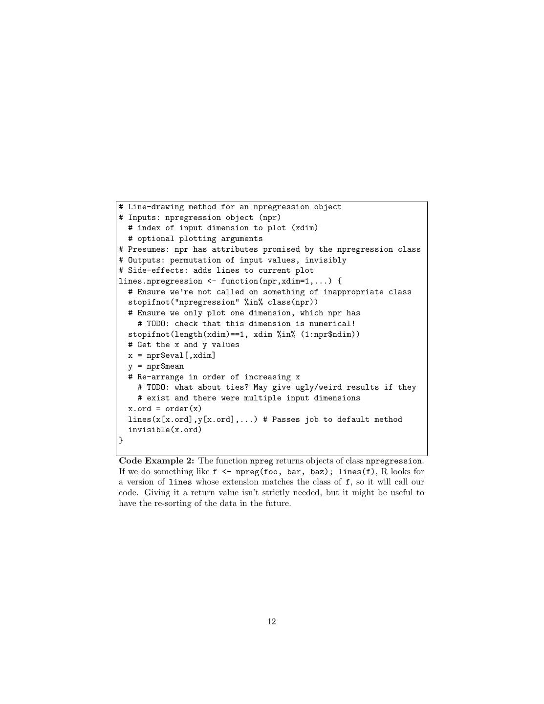
12 .# Line-drawing method for an npregression object # Inputs: npregression object (npr) # index of input dimension to plot (xdim) # optional plotting arguments # Presumes: npr has attributes promised by the npregression class # Outputs: permutation of input values, invisibly # Side-effects: adds lines to current plot lines.npregression <- function(npr,xdim=1,...) { # Ensure we’re not called on something of inappropriate class stopifnot("npregression" %in% class(npr)) # Ensure we only plot one dimension, which npr has # TODO: check that this dimension is numerical! stopifnot(length(xdim)==1, xdim %in% (1:npr$ndim)) # Get the x and y values x = npr$eval[,xdim] y = npr$mean # Re-arrange in order of increasing x # TODO: what about ties? May give ugly/weird results if they # exist and there were multiple input dimensions x.ord = order(x) lines(x[x.ord],y[x.ord],...) # Passes job to default method invisible(x.ord) } Code Example 2: The function npreg returns objects of class npregression. If we do something like f <- npreg(foo, bar, baz); lines(f), R looks for a version of lines whose extension matches the class of f, so it will call our code. Giving it a return value isn’t strictly needed, but it might be useful to have the re-sorting of the data in the future. 12 

13 .# Pick npreg bandwidth by k-fold CV and then use it # Inputs: vector of input feature values (x) # vector of response values (y) # vector of bandwidths (bandwidths) # fraction of data for each training set (training.fraction) # number of folds (folds) # optional extra arguments to npreg (...) # Calls: cv_bws_npreg, npreg # Ouputs: fitted npregression object cv_npreg <- function(x,y,bandwidths=(1:50)/50, training.fraction=0.9,folds=10,...) { cv <- cv_bws_npreg(x,y,bandwidths,training.fraction,folds) fit <- npreg(bws=cv$best.bw,txdat=x,tydat=y,...) return(fit) } Code Example 3: Combining k-fold CV bandwidth selection and npreg fitting into one function. Discards the details of the cross-validation; we could add that information as extra attributes to the return value, however. 13 

14 .2 Testing Functional Forms One important, but under-appreciated, use of nonparametric regression is in testing whether parametric regressions are well-specified. The typical parametric regression model is something like Y = f (X; θ) + (4) where f is some function which is completely specified except for the adjustable parameters θ, and , as usual, is uncorrelated noise. Overwhelmingly, f is linear in the variables in X, or perhaps includes some interactions between them. How can we tell if the specification is right? If, for example, it’s a linear model, how can we check whether there might not be some nonlinearity? One common approach is to modify the specification by adding in specific departures from the modeling assumptions — say, adding a quadratic term — and seeing whether the coefficients that go with those terms are significantly non-zero, or whether the improvement in fit is significant.6 For example, one might compare the model Y = θ1 x1 + θ2 x2 + (5) to the model Y = θ1 x1 + θ2 x2 + θ3 x21 + (6) by checking whether the estimated θ3 is significantly different from 0, or whether the residuals from the second model are significantly smaller than the residuals from the first. This can work, if you have chosen the right nonlinearity to test. It has the power to detect certain mis-specifications, if they exist, but not others. (What if the departure from linearity is not quadratic but cubic?) If you have good reasons to think that if the model is wrong, it can only be wrong in certain ways, fine; if not, though, why only check for those errors? Nonparametric regression effectively lets you check for all kinds of system- atic errors, rather than singling out a particular one. There are three basic approaches, which I give in order of increasing sophistication. • If the parametric model is right, it should predict as well as the non- parametric one, we can check whether M SEp (θ) − M SEnp (r) is approxi- mately zero. • If the parametric model is right, the non-parametric estimated regression curve should be very close to the parametric one. So we can check whether f (x; θ) − r(x) is approximately zero everywhere. • If the parametric model is right, then its residuals should be pattern- less and independent of input features. So we can apply non-parametric smoothing to the parametric residuals, y − f (x; θ), and see if they are approximately zero with constant variance everywhere. (Or, if the para- metric model is heteroskedastic, with the specified variance.) 6 In my experience, this is second in popularity only to ignoring the issue. 14 

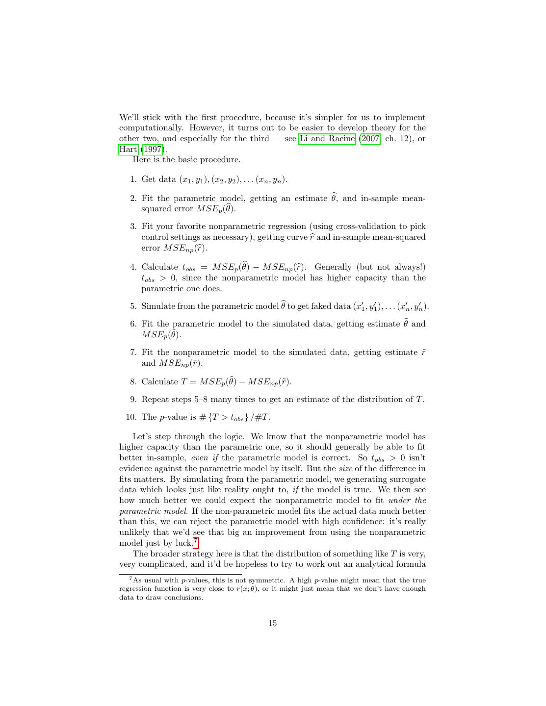
15 .We’ll stick with the first procedure, because it’s simpler for us to implement computationally. However, it turns out to be easier to develop theory for the other two, and especially for the third — see Li and Racine (2007, ch. 12), or Hart (1997). Here is the basic procedure. 1. Get data (x1 , y1 ), (x2 , y2 ), . . . (xn , yn ). 2. Fit the parametric model, getting an estimate θ, and in-sample mean- squared error M SEp (θ). 3. Fit your favorite nonparametric regression (using cross-validation to pick control settings as necessary), getting curve r and in-sample mean-squared error M SEnp (r). 4. Calculate tobs = M SEp (θ) − M SEnp (r). Generally (but not always!) tobs > 0, since the nonparametric model has higher capacity than the parametric one does. 5. Simulate from the parametric model θ to get faked data (x1 , y1 ), . . . (xn , yn ). 6. Fit the parametric model to the simulated data, getting estimate θ˜ and ˜ M SEp (θ). 7. Fit the nonparametric model to the simulated data, getting estimate r˜ and M SEnp (˜ r). ˜ − M SEnp (˜ 8. Calculate T = M SEp (θ) r). 9. Repeat steps 5–8 many times to get an estimate of the distribution of T . 10. The p-value is # {T > tobs } /#T . Let’s step through the logic. We know that the nonparametric model has higher capacity than the parametric one, so it should generally be able to fit better in-sample, even if the parametric model is correct. So tobs > 0 isn’t evidence against the parametric model by itself. But the size of the difference in fits matters. By simulating from the parametric model, we generating surrogate data which looks just like reality ought to, if the model is true. We then see how much better we could expect the nonparametric model to fit under the parametric model. If the non-parametric model fits the actual data much better than this, we can reject the parametric model with high confidence: it’s really unlikely that we’d see that big an improvement from using the nonparametric model just by luck.7 The broader strategy here is that the distribution of something like T is very, very complicated, and it’d be hopeless to try to work out an analytical formula 7 As usual with p-values, this is not symmetric. A high p-value might mean that the true regression function is very close to r(x; θ), or it might just mean that we don’t have enough data to draw conclusions. 15 

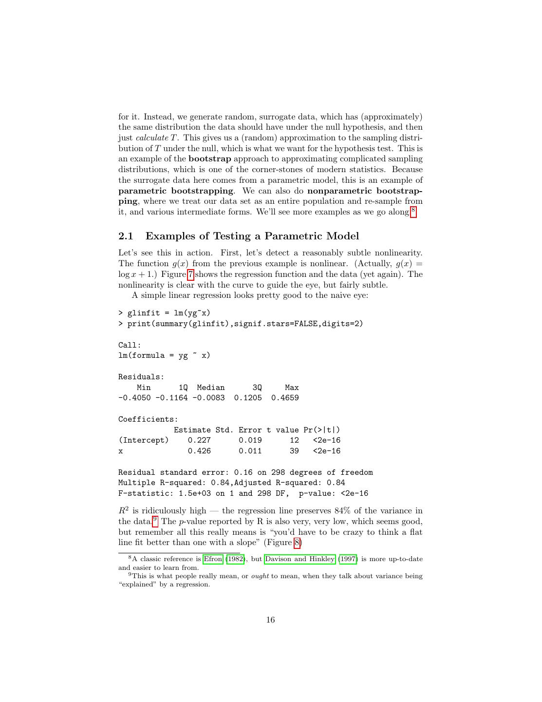
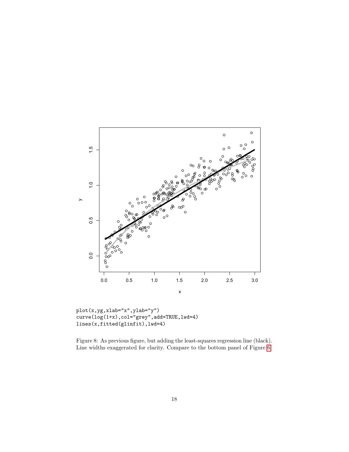
16 .for it. Instead, we generate random, surrogate data, which has (approximately) the same distribution the data should have under the null hypothesis, and then just calculate T . This gives us a (random) approximation to the sampling distri- bution of T under the null, which is what we want for the hypothesis test. This is an example of the bootstrap approach to approximating complicated sampling distributions, which is one of the corner-stones of modern statistics. Because the surrogate data here comes from a parametric model, this is an example of parametric bootstrapping. We can also do nonparametric bootstrap- ping, where we treat our data set as an entire population and re-sample from it, and various intermediate forms. We’ll see more examples as we go along.8 2.1 Examples of Testing a Parametric Model Let’s see this in action. First, let’s detect a reasonably subtle nonlinearity. The function g(x) from the previous example is nonlinear. (Actually, g(x) = log x + 1.) Figure 7 shows the regression function and the data (yet again). The nonlinearity is clear with the curve to guide the eye, but fairly subtle. A simple linear regression looks pretty good to the naive eye: > glinfit = lm(yg~x) > print(summary(glinfit),signif.stars=FALSE,digits=2) Call: lm(formula = yg ~ x) Residuals: Min 1Q Median 3Q Max -0.4050 -0.1164 -0.0083 0.1205 0.4659 Coefficients: Estimate Std. Error t value Pr(>|t|) (Intercept) 0.227 0.019 12 <2e-16 x 0.426 0.011 39 <2e-16 Residual standard error: 0.16 on 298 degrees of freedom Multiple R-squared: 0.84,Adjusted R-squared: 0.84 F-statistic: 1.5e+03 on 1 and 298 DF, p-value: <2e-16 R2 is ridiculously high — the regression line preserves 84% of the variance in the data.9 The p-value reported by R is also very, very low, which seems good, but remember all this really means is “you’d have to be crazy to think a flat line fit better than one with a slope” (Figure 8) 8 A classic reference is Efron (1982), but Davison and Hinkley (1997) is more up-to-date and easier to learn from. 9 This is what people really mean, or ought to mean, when they talk about variance being “explained” by a regression. 16 

17 . 1.5 1.0 y 0.5 0.0 0.0 0.5 1.0 1.5 2.0 2.5 3.0 x par(mfcol=c(1,1)) plot(x,yg,xlab="x",ylab="y") curve(log(1+x),col="grey",add=TRUE) Figure 7: True regression curve (grey) and data points (circles). The curve g(x) = log x + 1. 17 

18 . 1.5 1.0 y 0.5 0.0 0.0 0.5 1.0 1.5 2.0 2.5 3.0 x plot(x,yg,xlab="x",ylab="y") curve(log(1+x),col="grey",add=TRUE,lwd=4) lines(x,fitted(glinfit),lwd=4) Figure 8: As previous figure, but adding the least-squares regression line (black). Line widths exaggerated for clarity. Compare to the bottom panel of Figure 6. 18 

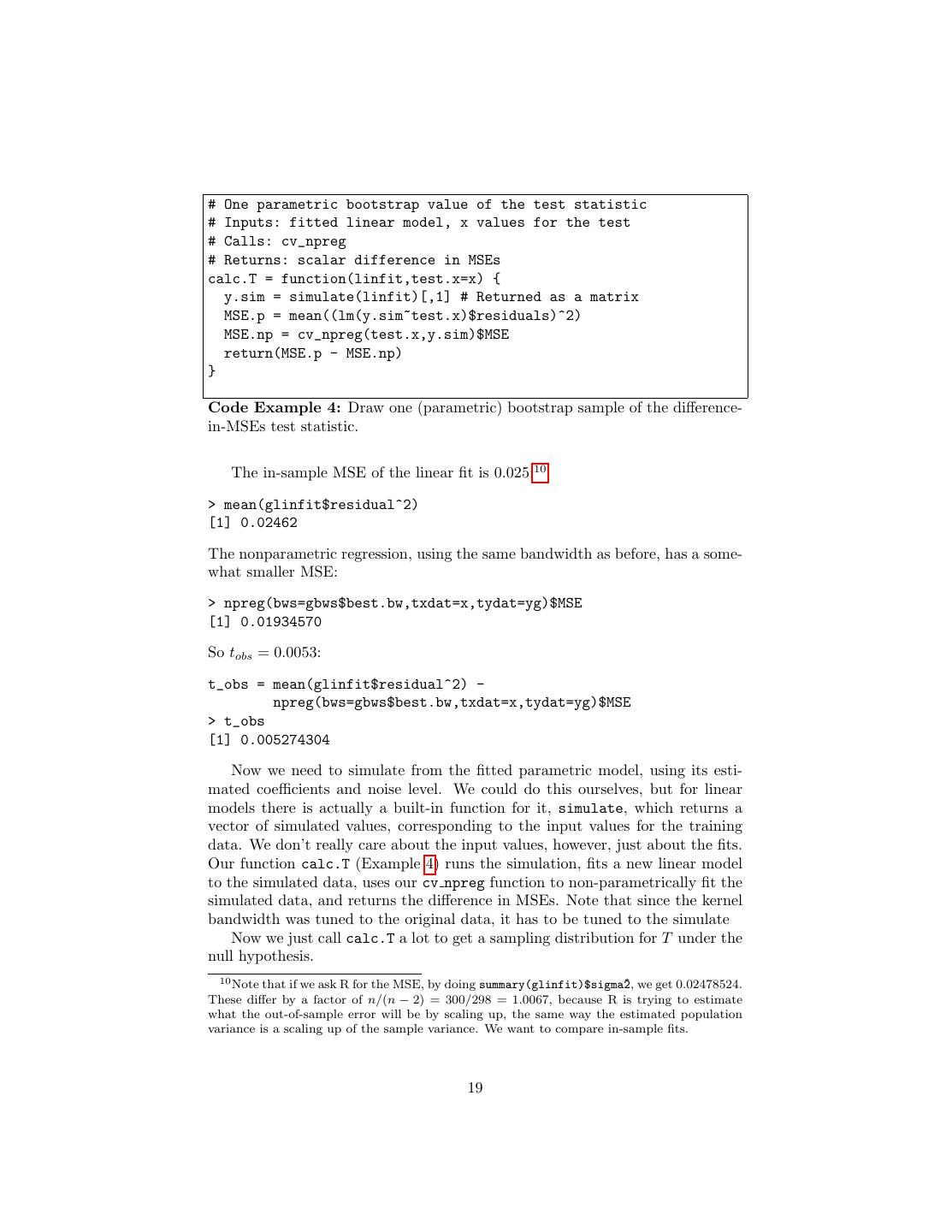
19 .# One parametric bootstrap value of the test statistic # Inputs: fitted linear model, x values for the test # Calls: cv_npreg # Returns: scalar difference in MSEs calc.T = function(linfit,test.x=x) { y.sim = simulate(linfit)[,1] # Returned as a matrix MSE.p = mean((lm(y.sim~test.x)$residuals)^2) MSE.np = cv_npreg(test.x,y.sim)$MSE return(MSE.p - MSE.np) } Code Example 4: Draw one (parametric) bootstrap sample of the difference- in-MSEs test statistic. The in-sample MSE of the linear fit is 0.025:10 > mean(glinfit$residual^2) [1] 0.02462 The nonparametric regression, using the same bandwidth as before, has a some- what smaller MSE: > npreg(bws=gbws$best.bw,txdat=x,tydat=yg)$MSE [1] 0.01934570 So tobs = 0.0053: t_obs = mean(glinfit$residual^2) - npreg(bws=gbws$best.bw,txdat=x,tydat=yg)$MSE > t_obs [1] 0.005274304 Now we need to simulate from the fitted parametric model, using its esti- mated coefficients and noise level. We could do this ourselves, but for linear models there is actually a built-in function for it, simulate, which returns a vector of simulated values, corresponding to the input values for the training data. We don’t really care about the input values, however, just about the fits. Our function calc.T (Example 4) runs the simulation, fits a new linear model to the simulated data, uses our cv npreg function to non-parametrically fit the simulated data, and returns the difference in MSEs. Note that since the kernel bandwidth was tuned to the original data, it has to be tuned to the simulate Now we just call calc.T a lot to get a sampling distribution for T under the null hypothesis. 10 Note that if we ask R for the MSE, by doing summary(glinfit)$sigma^ 2, we get 0.02478524. These differ by a factor of n/(n − 2) = 300/298 = 1.0067, because R is trying to estimate what the out-of-sample error will be by scaling up, the same way the estimated population variance is a scaling up of the sample variance. We want to compare in-sample fits. 19 

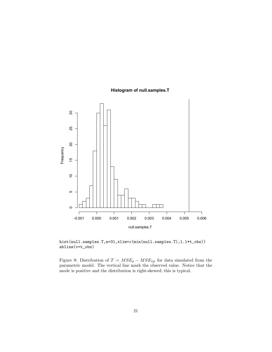
20 .null.samples.T <- replicate(200,calc.T(glinfit)) This takes some time, because each replication involves not just generating a new simulation sample, but also using ten-fold cross-validation to pick a band- width, which means that the simulated data undergoes ten random divisions into training and testing sets. This adds up to about 10 seconds per replicate on my laptop, and about half an hour for the whole deal. (While the computer is thinking, look at the command a little more closely. It leaves the x values alone, and only uses simulation to generate new y values. This is appropriate here because our model doesn’t really say where the x values came from; it’s just about the conditional distribution of Y given X. If the model we were testing specified a distribution for x, we should generate x each time we invoke calc.T. If the specification is vague, like “x is IID” but with no particular distribution, then use the bootstrap. The command would be something like replicate(1000,calc.T(glinfit,sample(x,size=length(x),replace=TRUE))) to draw a different bootstrap sample of x each time. But we’d have to modify the internals of calc.T to simulate at the appropriate places.) When it’s done, we can plot the distribution and see that the observed value tobs is pretty far out along the right tail (Figure 9). This tells us that it’s very unlikely that npreg would improve so much on the linear model if the latter were true. In fact, none of the bootstrap replicates were that big: > sum(null.samples.T > t_obs) [1] 0 so we can conclude p < 1/200. We can thus reject the linear model pretty confidently. As a second example, let’s suppose that the linear model is right — then the test should give us a high p-value. So let us stipulate that in reality Y = 0.2 + 0.5x + η (7) with η ∼ N (0, 0.152 ). Figure 10 shows data from this, of the same size as before. Repeating the same exercise as before, we get that tobs = 0.00064, together with a slightly different null distribution (Figure 11). Now the p-value is 45%, which one would be quite rash to reject. 2.2 Why Use Parametric Models At All? It might seem by this point that there is little point to using parametric models at all. Either our favorite parametric model is right, or it isn’t. If it is right, then a consistent nonparametric estimate will eventually approximate it arbitrarily closely. If the parametric model is wrong, it will not self-correct, but the non- parametric estimate will eventually show us that the parametric model doesn’t work. Either way, the parametric model seems superfluous. 20 

21 . Histogram of null.samples.T 30 25 20 Frequency 15 10 5 0 -0.001 0.000 0.001 0.002 0.003 0.004 0.005 0.006 null.samples.T hist(null.samples.T,n=31,xlim=c(min(null.samples.T),1.1*t_obs)) abline(v=t_obs) Figure 9: Distribution of T = M SEp − M SEnp for data simulated from the parametric model. The vertical line mark the observed value. Notice that the mode is positive and the distribution is right-skewed; this is typical. 21 

22 . 2.0 1.5 1.0 y 0.5 0.0 0.0 0.5 1.0 1.5 2.0 2.5 3.0 x y2 = 0.2+0.5*x + rnorm(length(x),0,0.15) plot(x,y2,xlab="x",ylab="y") abline(0.2,0.5,col="grey") Figure 10: Data from the linear model (true regression line in grey). 22 

23 . Histogram of null.samples.T 25 20 Frequency 15 10 5 0 -0.001 0.000 0.001 0.002 0.003 0.004 null.samples.T Figure 11: As in Figure 9, but using the data and fits from Figure 10. 23 

24 .nearly.linear.out.of.sample = function(n) { x=seq(from=0,to=3,length.out=n) y = h(x) + rnorm(n,0,0.15) y.new = h(x) + rnorm(n,0,0.15) lm.mse = mean(( fitted(lm(y~x)) - y.new )^2) np.mse = mean((cv_npreg(x,y)$mean - y.new)^2) return(c(lm.mse,np.mse)) } nearly.linear.generalization = function(n,m=100) { raw = replicate(m,nearly.linear.out.of.sample(n)) reduced = rowMeans(raw) return(reduced) } Code Example 5: Evaluating the out-of-sample error for the nearly-linear problem as a function of n, and evaluting the generalization error by averaging over many samples. There is an escape from this dilemma, by means of the bias-variance trade- off.11 Low-dimensional parametric models have potentially high bias (if the real regression curve is very different from what the model posits), but low variance (because there isn’t that much to estimate). Non-parametric regression models have low bias (they’re flexible) but high variance (they’re flexible). If the parametric model is true, it can converge faster than the non-parametric one. Even if the parametric model isn’t quite true, the lower variance can still make it beat out the non-parametric model in over-all generalization error. To illustrate, suppose that the true regression function is 1 sin x E [Y |X = x] = 0.2 + 1+ x (8) 2 10 This is very nearly linear over small ranges — say x ∈ [0, 3] (Figure 12). I will use the fact that I know the true model here to calculate the actual expected generalization error, by averaging over many samples (Example 5). Figure 13 shows that, out to a fairly substantial sample size (≈ 500), the lower bias of the non-parametric regression is systematically beaten by the lower variance of the linear model — though admittedly not by much. 11 Actually, there is another way out as well. If the parametric model actually represents our idea about the mechanism generating the data, then its parameters are substantively, “physically” meaningful and interesting, and the non-parametric smoothing doesn’t capture that. However, this situation is so rare in data mining, as opposed to scientific inference, that I won’t go further into this. 24 

25 . 1.5 1.0 h(x) 0.5 0.0 0.5 1.0 1.5 2.0 2.5 3.0 x 1 sin x Figure 12: Graph of h(x) = 0.2 + 2 1+ 10 x over [0, 3]. 25 

26 . 0.20 0.15 RMS generalization error 0.10 0.05 0.00 0 100 200 300 400 500 n sizes = c(5,10,15,20,25,30,50,100,200,500) generalizations = sapply(sizes,nearly.linear.generalization) plot(sizes,sqrt(generalizations[1,]),ylim=c(0,0.22),type="l", xlab="n",ylab="RMS generalization error") lines(sizes,sqrt(results[2,]),lty=2) Figure 13: Root-mean-square generalization error for linear model (solid line) and kernel smoother (dashed line), fit to the same sample of the indicated size. The true regression curve is as in 12, and observations are corrupted by IID Gaussian noise with σ = 0.15. The cross-over after which the nonparametric regressor has better generalization performance happens shortly before n = 500. 26 

27 .References Davison, A. C. and D. V. Hinkley (1997). Bootstrap Methods and their Appli- cations. Cambridge, England: Cambridge University Press. Efron, Bradley (1982). The Jackknife, the Bootstrap, and Other Resampling Plans. Philadelphia: SIAM Press. Hart, Jeffrey D. (1997). Nonparametric Smoothing and Lack-of-Fit Tests. Springer Series in Statistics. Berlin: Springer-Verlag. Hayfield, Tristen and Jeffrey S. Racine (2008). “Nonparametric Econometrics: The np Package.” Journal of Statistical Software, 27(5): 1–32. URL http: //www.jstatsoft.org/v27/i05. Li, Qi and Jeffrey Scott Racine (2007). Nonparametric Econometrics: Theory and Practice. Princeton, New Jersey: Princeton University Press. 27