Regression III: Extending Linear Regression

1 . Extending Linear Regression: Weighted Least Squares, Heteroskedasticity, Local Polynomial Regression 36-350, Data Mining 23 October 2009 Contents 1 Weighted Least Squares 1 2 Heteroskedasticity 3 2.1 Weighted Least Squares as a Solution to Heteroskedasticity . . . 5 3 Local Linear Regression 10 4 Exercises 15 1 Weighted Least Squares Instead of minimizing the residual sum of squares, n RSS(β) = (yi − xi · β)2 (1) i=1 we could minimize the weighted sum of squares, n W SS(β, w) = wi (yi − xi · β)2 (2) i=1 This includes ordinary least squares as the special case where all the weights wi = 1. We can solve it by the same kind of algebra we used to solve the ordinary linear least squares problem. But why would we want to solve it? For three reasons. 1. Focusing accuracy. We may care very strongly about predicting the re- sponse for certain values of the input — ones we expect to see often again, ones where mistakes are especially costly or embarrassing or painful, etc. 1 

2 . — than others. If we give the points xi near that region big weights wi , and points elsewhere smaller weights, the regression will be pulled towards matching the data in that region. 2. Discounting imprecision. Ordinary least squares is the maximum likeli- hood estimate when the in Y = X · β + is IID Gaussian white noise. This means that the variance of has to be constant, and we measure the regression curve with the same precision elsewhere. This situation, of constant noise variance, is called homoskedasticity. Often however the magnitude of the noise is not constant, and the data are heteroskedastic. When we have heteroskedasticity, even if each noise term is still Gaussian, ordinary least squares is no longer the maximum likelihood estimate, and so no longer efficient. If however we know the noise variance σi2 at each measurement i, and set wi = 1/σi2 , we get the heteroskedastic MLE, and recover efficiency. To say the same thing slightly differently, there’s just no way that we can estimate the regression function as accurately where the noise is large as we can where the noise is small. Trying to give equal attention to all parts of the input space is a waste of time; we should be more concerned about fitting well where the noise is small, and expect to fit poorly where the noise is big. 3. Doing something else. There are a number of other optimization prob- lems which can be transformed into, or approximated by, weighted least squares. The most important of these arises from generalized linear mod- els, where the mean response is some nonlinear function of a linear pre- dictor. (Logistic regression is an example.) In the first case, we decide on the weights to reflect our priorities. In the third case, the weights come from the optimization problem we’d really rather be solving. What about the second case, of heteroskedasticity? 2 

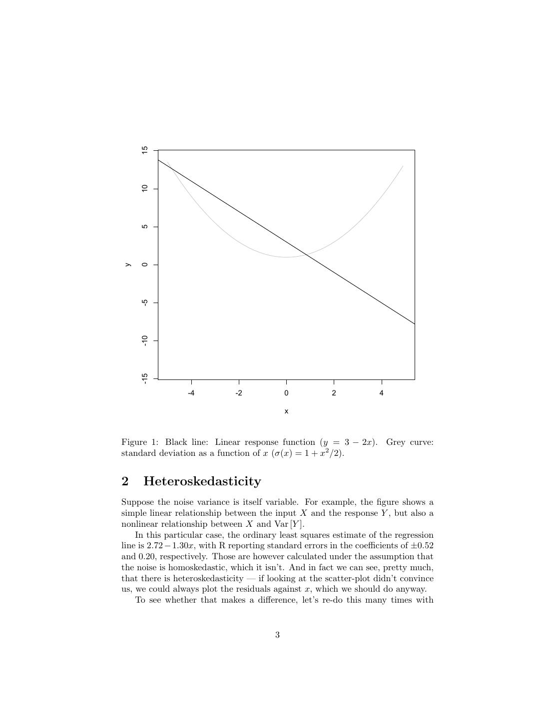
3 . 15 10 5 0 y -5 -10 -15 -4 -2 0 2 4 x Figure 1: Black line: Linear response function (y = 3 − 2x). Grey curve: standard deviation as a function of x (σ(x) = 1 + x2 /2). 2 Heteroskedasticity Suppose the noise variance is itself variable. For example, the figure shows a simple linear relationship between the input X and the response Y , but also a nonlinear relationship between X and Var [Y ]. In this particular case, the ordinary least squares estimate of the regression line is 2.72 − 1.30x, with R reporting standard errors in the coefficients of ±0.52 and 0.20, respectively. Those are however calculated under the assumption that the noise is homoskedastic, which it isn’t. And in fact we can see, pretty much, that there is heteroskedasticity — if looking at the scatter-plot didn’t convince us, we could always plot the residuals against x, which we should do anyway. To see whether that makes a difference, let’s re-do this many times with 3 

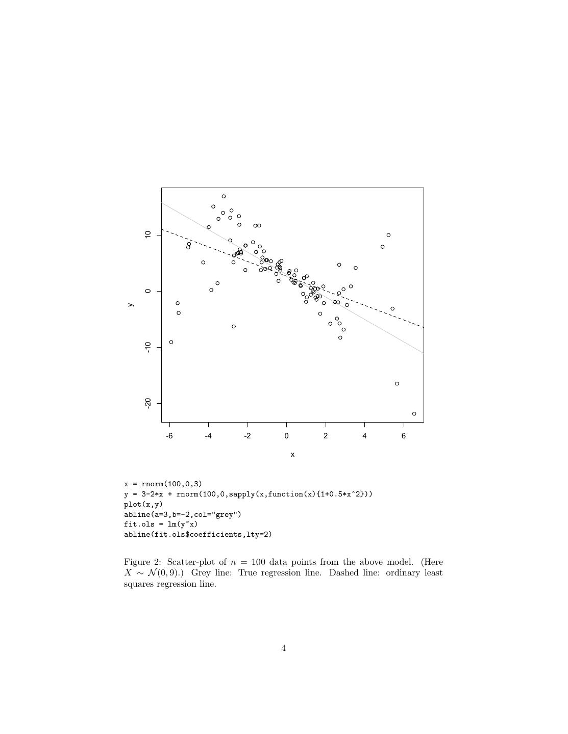
4 . 10 0 y -10 -20 -6 -4 -2 0 2 4 6 x x = rnorm(100,0,3) y = 3-2*x + rnorm(100,0,sapply(x,function(x){1+0.5*x^2})) plot(x,y) abline(a=3,b=-2,col="grey") fit.ols = lm(y~x) abline(fit.ols$coefficients,lty=2) Figure 2: Scatter-plot of n = 100 data points from the above model. (Here X ∼ N (0, 9).) Grey line: True regression line. Dashed line: ordinary least squares regression line. 4 

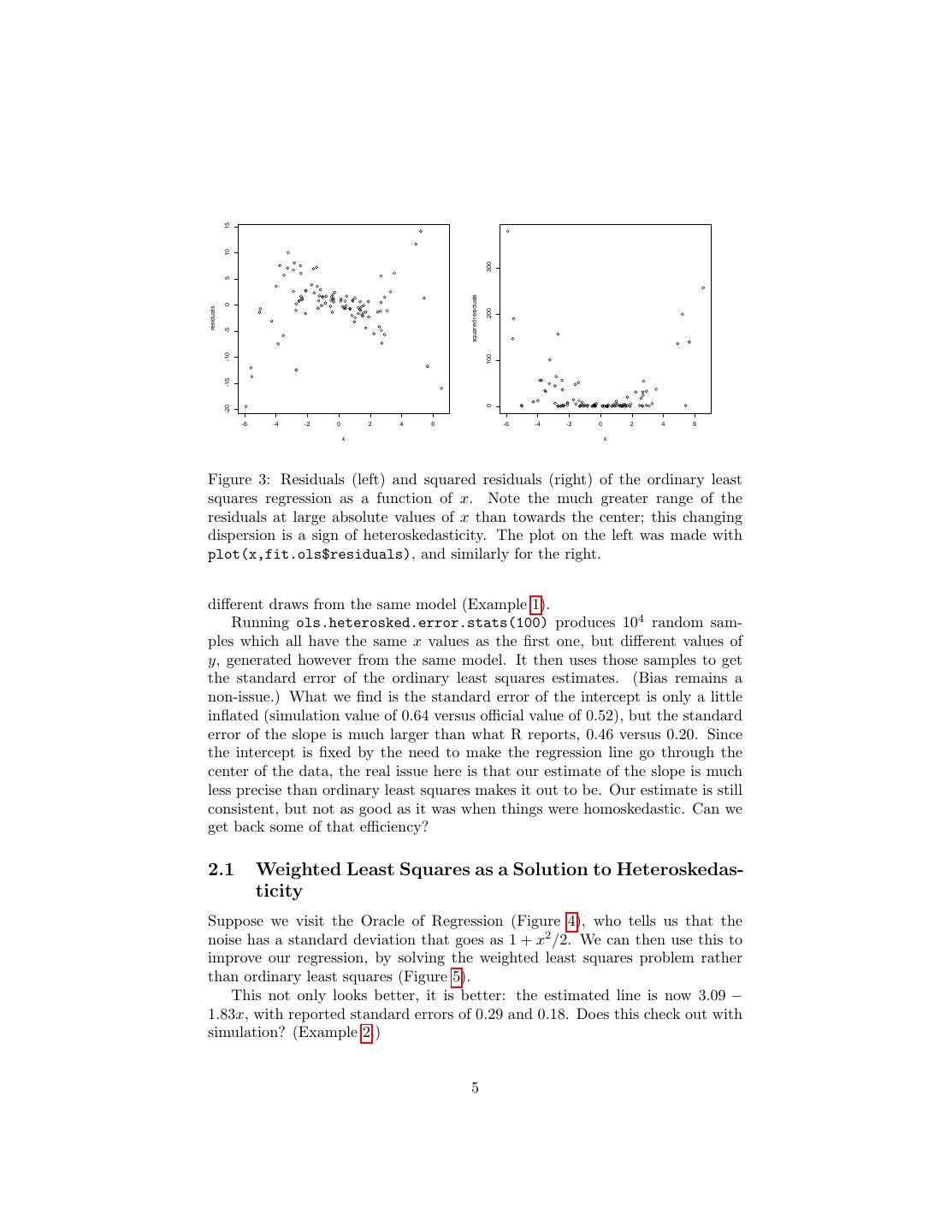
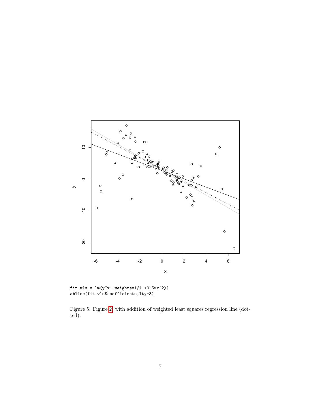
5 . 15 10 300 5 squared residuals 0 residuals 200 -5 -10 100 -15 0 -20 -6 -4 -2 0 2 4 6 -6 -4 -2 0 2 4 6 x x Figure 3: Residuals (left) and squared residuals (right) of the ordinary least squares regression as a function of x. Note the much greater range of the residuals at large absolute values of x than towards the center; this changing dispersion is a sign of heteroskedasticity. The plot on the left was made with plot(x,fit.ols$residuals), and similarly for the right. different draws from the same model (Example 1). Running ols.heterosked.error.stats(100) produces 104 random sam- ples which all have the same x values as the first one, but different values of y, generated however from the same model. It then uses those samples to get the standard error of the ordinary least squares estimates. (Bias remains a non-issue.) What we find is the standard error of the intercept is only a little inflated (simulation value of 0.64 versus official value of 0.52), but the standard error of the slope is much larger than what R reports, 0.46 versus 0.20. Since the intercept is fixed by the need to make the regression line go through the center of the data, the real issue here is that our estimate of the slope is much less precise than ordinary least squares makes it out to be. Our estimate is still consistent, but not as good as it was when things were homoskedastic. Can we get back some of that efficiency? 2.1 Weighted Least Squares as a Solution to Heteroskedas- ticity Suppose we visit the Oracle of Regression (Figure 4), who tells us that the noise has a standard deviation that goes as 1 + x2 /2. We can then use this to improve our regression, by solving the weighted least squares problem rather than ordinary least squares (Figure 5). This not only looks better, it is better: the estimated line is now 3.09 − 1.83x, with reported standard errors of 0.29 and 0.18. Does this check out with simulation? (Example 2.) 5 

6 .ols.heterosked.example = function(n) { y = 3-2*x + rnorm(n,0,sapply(x,function(x){1+0.5*x^2})) fit.ols = lm(y~x) # Return the errors return(fit.ols$coefficients - c(3,-2)) } ols.heterosked.error.stats = function(n,m=10000) { ols.errors.raw = t(replicate(m,ols.heterosked.example(n))) # transpose gives us a matrix with named columns intercept.sd = sd(ols.errors.raw[,"(Intercept)"]) slope.sd = sd(ols.errors.raw[,"x"]) return(list(intercept.sd=intercept.sd,slope.sd=slope.sd)) } Code Example 1: Functions to generate heteroskedastic data and fit OLS regression to it, and to collect error statistics on the results. Figure 4: Statistician (right) consulting the Oracle of Regression (left) about the proper weights to use to overcome heteroskedasticity. (Image from http://en.wikipedia. org/wiki/Image:Pythia1.jpg.) 6 

7 . 10 0 y -10 -20 -6 -4 -2 0 2 4 6 x fit.wls = lm(y~x, weights=1/(1+0.5*x^2)) abline(fit.wls$coefficients,lty=3) Figure 5: Figure 2, with addition of weighted least squares regression line (dot- ted). 7 

8 .wls.heterosked.example = function(n) { y = 3-2*x + rnorm(n,0,sapply(x,function(x){1+0.5*x^2})) fit.wls = lm(y~x,weights=1/(1+0.5*x^2)) # Return the errors return(fit.wls$coefficients - c(3,-2)) } wls.heterosked.error.stats = function(n,m=10000) { wls.errors.raw = t(replicate(m,wls.heterosked.example(n))) # transpose gives us a matrix with named columns intercept.sd = sd(wls.errors.raw[,"(Intercept)"]) slope.sd = sd(wls.errors.raw[,"x"]) return(list(intercept.sd=intercept.sd,slope.sd=slope.sd)) } Code Example 2: Linear regression of heteroskedastic data, using weighted least-squared regression. The standard errors from the simulation are 0.22 for the intercept and 0.23 for the slope, so R’s internal calculations are working very well. All of this was possible because the Oracle told us what the variance function was. What do we do when the Oracle is not available (Figure 6)? Under some situations we can work things out for ourselves, without needing an oracle. • We know, empirically, the precision of our measurement of the response variable — we know how precise our instruments are, or each value of the response is really an average of several measurements so we can use their standard deviations, etc. • We know how the noise in the response must depend on the input variables. For example, when taking polls or surveys, the variance of the proportions we find should be inversely proportional to the sample size. So we can make the weights proportional to the sample size. Both of these outs rely on kinds of background knowledge which are easier to get in the natural or even the social sciences than in data mining applications. However, there are approaches for other situations which try to use the observed residuals to get estimates of the heteroskedasticity. This can then go into a weighted regression, and so forth; let me just sketch the idea for how to get the variance function in the first place1 . 1. Estimate r(x) with your favorite regression method, getting rˆ(x). 2 2. Construct the log squared residuals, zi = log (yi − rˆ(xi )) ). 1 This is ripped off from Wasserman (2006, pp. 87–88). 8 

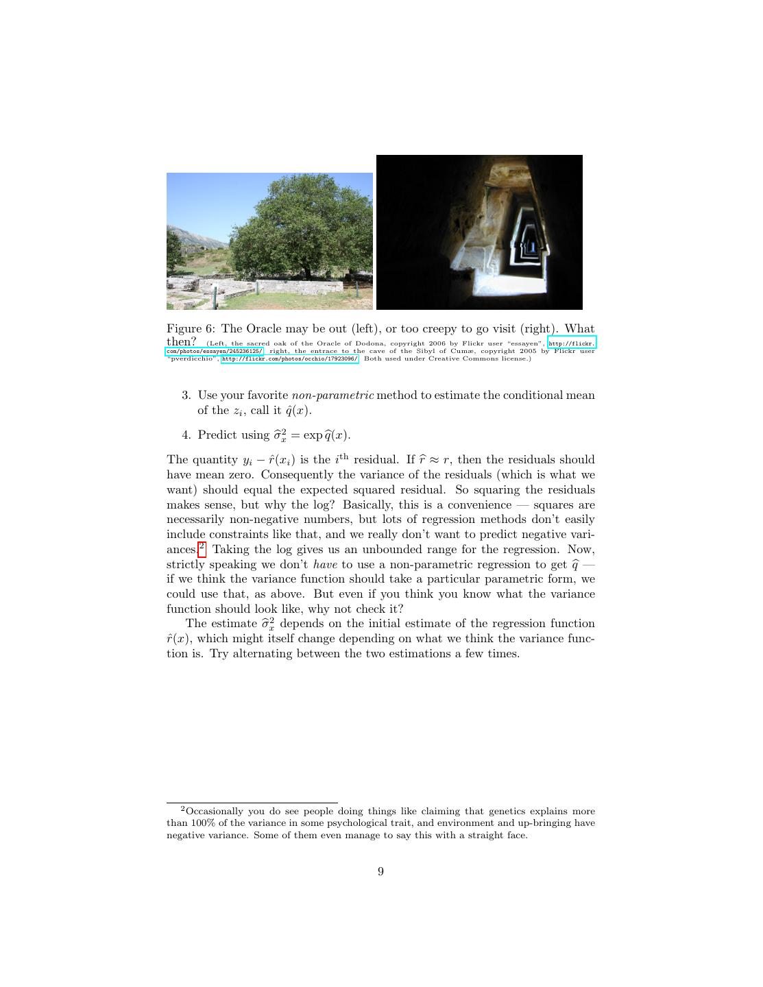
9 .Figure 6: The Oracle may be out (left), or too creepy to go visit (right). What then? (Left, the sacred oak of the Oracle of Dodona, copyright 2006 by Flickr user “essayen”, http://flickr. com/photos/essayen/245236125/; right, the entrace to the cave of the Sibyl of Cumæ, copyright 2005 by Flickr user “pverdicchio”, http://flickr.com/photos/occhio/17923096/. Both used under Creative Commons license.) 3. Use your favorite non-parametric method to estimate the conditional mean of the zi , call it qˆ(x). 4. Predict using σx2 = exp q(x). The quantity yi − rˆ(xi ) is the ith residual. If r ≈ r, then the residuals should have mean zero. Consequently the variance of the residuals (which is what we want) should equal the expected squared residual. So squaring the residuals makes sense, but why the log? Basically, this is a convenience — squares are necessarily non-negative numbers, but lots of regression methods don’t easily include constraints like that, and we really don’t want to predict negative vari- ances.2 Taking the log gives us an unbounded range for the regression. Now, strictly speaking we don’t have to use a non-parametric regression to get q — if we think the variance function should take a particular parametric form, we could use that, as above. But even if you think you know what the variance function should look like, why not check it? The estimate σx2 depends on the initial estimate of the regression function rˆ(x), which might itself change depending on what we think the variance func- tion is. Try alternating between the two estimations a few times. 2 Occasionally you do see people doing things like claiming that genetics explains more than 100% of the variance in some psychological trait, and environment and up-bringing have negative variance. Some of them even manage to say this with a straight face. 9 

10 .3 Local Linear Regression Switching gears, recall from the last handout that one reason it can be sensible to use a linear approximation to the true regression function r(x) is that we can always3 Taylor-expand the latter around any point x0 , ∞ k (x − x0 ) dk r r(x) = r(x0 ) + (3) k! drk x=x0 k=1 and similarly with all the partial derivatives in higher dimensions. If we truncate the series at first order, r(x) ≈ r(x0 ) + (x − x0 )r (x0 ), we see that the first-order coefficient r (x0 ) is the best linear prediction coefficient, at least when x is sufficiently close to x0 . The snag in this line of argument is that if r(x) isn’t really linear, then r isn’t a constant, and the optimal linear predictor to use depends on where we want to make predictions. However, statisticians are thrifty people, and having assembled all the ma- chinery for linear regression, they are loathe to throw it away just because the fundamental model is wrong. If we can’t fit one line, why not fit many? If each point has a different best linear regression, why not estimate them all? Thus the idea of local linear regression: fit a different linear regression everywhere, weighting the data points by how close they are to the point of interest. The simplest approach you could imagine would be to take a window of some fixed width (say, 2h) around the point of interest (call it x0 for concreteness) and include only the data points which fell within that window. This is a weighted least-squares regression with wi = 1 if |xi − x0 | < h and wi = 0 if |xi − x0 | ≥ h. This is however cruder than it needs to be. Remember that the reason we’re doing this is that observations near x0 are supposed to tell us more about the slope at x0 than points which are far from it; but the simple 0/1 weighting does this in a very rough way. It generally works nicer to have the weights change more smoothly with the distance, starting off large and then gradually trailing to zero. By now bells may be going off in your head, as this sounds very similar to the kernel regression or Nadaraya-Watson regression from the last handout. In fact, kernel regression is what happens when we truncate Eq. 3 at zeroth order, getting locally constant regression. Here’s the problem we’re setting up: n 2 min wi (x)(yi − β(x)) β i=1 which has the solution n i=1 wi (x)yi β(x) = n j=1 wj (x) which just is our kernel regression from last time, with the weights being pro- portional to the kernels, wi (x) ∝ K(xi , x). (Without loss of generality, we can take the constant of proportionality to be 1.) 3 At least if r(x) is differentiable. 10 

11 . 1.0 0.8 0.6 tricubic function 0.4 0.2 0.0 -1.0 -0.5 0.0 0.5 1.0 x curve((1-abs(x)^3)^3,from=-1,to=1,ylab="tricubic function") Figure 7: The tricubic weighting function typically used in local linear regres- sion. Note the broad plateau where |x| ≈ 0, and the smooth fall-off to zero at |x| = 1. What about locally linear regression? The optimization problem is n 2 min wi (x)(yi − x · β(x)) β i=1 where again we can write wi (x) is proportional to some kernel function, wi (x) ∝ K(xi , x). For locally linear regression, a common choice of kernel tri-cubic, 3 3 |xi − x0 | K(xi , x) = 1− h if |x − xi | < h, and = 0 otherwise (Figure 7). This is what is used in the form of local linear regression called lowess or loess.4 Other kernels are certainly possible — there’s nothing magic about this one — but this works pretty reliably. Lowess smoothing is implemented in the default R packages through the function lowess (rather basic), and through the function loess (more sophis- ticated), as well as in the CRAN package locfit (more sophisticated still). In lowess, instead of specifying the actual width of the window, one specifies what fraction f of the data points should be included. Figure 3 shows lowess fits to data from the nonlinear model Y |X ∼ N (sin 10X, 1). With the right f , this can do a quite creditable job of recovering the underlying nonlinear regression 4 I have heard this name explained as an acronym for both “locally weighted scatterplot smoothing” and “locally weight sum of squares”. 11 

12 .function. On the other hand, if we choose the wrong f our results are not so good. The Oracle could tell us what f to use; we will see later what to do when we can’t find an oracle. Figure 9 shows some local linear fits to our running example, again varying f . All of the local linear fits seem to be better than ordinary least squares. In fact, the true regression line is kind of hard to see under the f = 1 local linear fit. Once we’ve figured out this localization trick once, we could apply it to any global fitting method. In particular, local polynomial fitting is pretty much as straightforward as local linear fitting. The loess and locfit commands support controlling the degree of the polynomial; lowess does not. 12 

13 . 3 2 1 y 0 -1 -2 0.0 0.2 0.4 0.6 0.8 1.0 x x.sin = runif(100,0,1) y.sin = sin(10*x.sin) + rnorm(100,0,1) plot(x.sin,y.sin,xlab="x",ylab="y");curve(sin(10*x),col="grey",add=TRUE) lines(lowess(x.sin,y.sin,f=1/3),lty=1) lines(lowess(x.sin,y.sin,f=2/3),lty=2) lines(lowess(x.sin,y.sin,f=1/6),lty=3) Figure 8: Samples from the model X ∼ Unif(0, 1), Y |X ∼ N (sin 10X, 1). The true regression function is the grey sine curve. Overlaid are lowess fits using different fractions f of the data at each point: solid line, f = 1/3; dashed line, f = 2/3 (default); dotted line, f = 1/6. 13 

14 . 10 0 y -10 -20 -6 -4 -2 0 2 4 6 x plot(x,y) abline(3,-2,col="grey") abline(fit.ols$coefficients,col="red") lines(lowess(x,y,f=2/3),lty=1) lines(lowess(x,y,f=1/3),lty=2) lines(lowess(x,y,f=3/4),lty=3) lines(lowess(x,y,f=1),lty=4) Figure 9: Running-example data, together with the true regression line (solid grey) and ordinary least-squares line (red), plus lowess fits using different frac- tions f of the data at each point. Solid line: f = 2/3 (default setting); Dashed line: f = 1/3; dotted line, f = 3/4; dot-dash line: f = 1. Note that the f = 1 lowess curve is not the same as the ordinary least squares line, because of the tri-cubic weighting. 14 

15 .4 Exercises 1. Find the β which minimizes Eq. 2 in terms of the data matrices X and Y, and the weights. Hint: consider the matrix w where wij = wi δij , and imitate the solution to the ordinary least squares problem. 2. Is wi = 1 a necessary as well as a sufficient condition for Eq. 2 and Eq. 1 to have the same minimum? 3. Should local linear regression do better or worse than ordinary least squares under heteroskedasticity? What exactly would this mean, and how might you test your ideas? References Wasserman, Larry (2006). All of Nonparametric Statistics. Berlin: Springer- Verlag. 15