信息理论II

1 . Information and Interaction Among Features 36-350: Data Mining 9 September 2009 Reading: Aleks Jakulin and Ivan Bratko, “Quantifying and Visualizing Attribute Interactions”, http://arxiv.org/abs/cs.AI/0308002 Contents 1 Entropy for Multiple Variables 2 2 Information in Multiple Variables 2 2.1 Example Calculation . . . . . . . . . . . . . . . . . . . . . . . . . 3 3 Conditional Information and Interaction 3 3.1 Interaction . . . . . . . . . . . . . . . . . . . . . . . . . . . . . . 4 3.2 The Chain Rule . . . . . . . . . . . . . . . . . . . . . . . . . . . . 4 4 Feature Selection with Mutual Information (Once More with Feeling) 5 4.1 Example for the Times Corpus . . . . . . . . . . . . . . . . . . . 6 4.1.1 Code . . . . . . . . . . . . . . . . . . . . . . . . . . . . . . 6 4.1.2 Results . . . . . . . . . . . . . . . . . . . . . . . . . . . . 11 5 Sufficient Statistics and the Information Bottleneck 14 Last time, I talked about using features to predict variables which are not immediately represented, like future events, or the category to which an object belongs. I gave you the machinery for saying how much entropy a single random variable has, and how much knowledge of one variable reduces the entropy of another — how much information they have about each other. I closed by talking about using this to select features. Basically, if you want to predict C and have features X1 , X2 , . . . Xp , calculate I[C; Xi ] for i = 1 : p, and take the most informative feature. Normally — and this is especially true when you have enough features that you want to do feature selection — you have many features, so we want a way to talk about using multiple features to predict C. You could just go down the list of informative features, but it’s easy to suspect this isn’t the right thing to do. Look at table 1 in the last lecture. “Painting” was the second most informative word, but “paintings” was number 6. Do you really think you’ll learn much 1 

2 .about the document from checking whether it has the word “paintings” if you already know whether it contains “painting”? Or looking for “music” after you’ve checked “orchestra”? Our subject for today, accordingly, is to extend the information theory we’ve seen to handle multiple features, and the idea that there can be interactions among features, that they can be more or less informative in different contexts. 1 Entropy for Multiple Variables The joint entropy of two random variables X and Y is just the entropy of their joint distribution: H[X, Y ] ≡ − Pr (X = x, Y = y) log2 Pr (X = x, Y = y) (1) x,y This definition extends naturally to the joint entropy of an arbitrary number of variables. A crucial property is that joint entropy is sub-additive: H[X, Y ] ≤ H[X] + H[Y ] (2) with equality if and only if X and Y are statistically independent. In terms of uncertainty, this says that you can’t be more uncertain about the pair (X, Y ) than you are about its components. In terms of coding, it says that the number of bits you need to encode the pair is no more than the number of bits you would need to encode each of its members. Again, this extends to any arbitrary number of variables. Conditional entropy and mutual information can both be defined in terms of the joint entropy: H[Y |X] = H[X, Y ] − H[X] (3) I[X; Y ] = H[X] + H[Y ] − H[X, Y ] (4) The last of these says that the mutual information is the difference between the joint entropy and the sum of the marginal entropies. This can be extended to any number of variables, giving what’s called the multi-information or higher-order mutual information, I[X; Y ; Z] = H[X] + H[Y ] + H[Z] − H[X, Y, Z] (5) (and so on for more than three variables). This is zero if and only if all the variables are statistically independent of each other. 2 Information in Multiple Variables If all we want is to know how much information a set of variables X1 , X2 , . . . Xk have about a given outcome or target variable C, that is just I[C; X1 , X2 , . . . Xk ] = H[C]+H[X1 , X2 , . . . Xk ]−H[C, X1 , X2 , . . . Xk ] = H[C]−H[C|X1 , X2 , . . . Xk ] (6) 2 

3 . It should not be hard to convince yourself that adding an extra variable increases joint entropy, decreases conditional entropy, and increases information: H[X, Y ] ≥ H[X] (7) H[C|X, Y ] ≤ H[C|X] (8) I[C; X, Y ] ≥ I[C; X] (9) and similarly with more predictor variables. 2.1 Example Calculation Let’s do an example. The single most informative word for our documents, we saw last time, is “art”, call its indicator X1 , followed by “painting” (say X2 ). How informative is the pair of words? To calculate this, we need a 2×2×2 (class × “art” × “painting”) contingency table, or alternately a 2 × 4 (class × (“art”, “painting”)) table. Because it’s easier to get two dimensions down on the page than three, I’ll use the latter right now, but we’ll switch later on, and you should get used to alternating between the two perspectives. “art” yes “art” no “painting” yes “painting” no “painting” yes “painting” no art 22 25 2 8 music 0 8 0 37 I’ll use the word.mutual.info function from last time: > art.painting.indicators <- matrix(c(22,25,2,8,0,8,0,37),byrow=TRUE,nrow=2) > word.mutual.info(art.painting.indicators) [1] 0.4335985 so I[C; X1 , X2 ] = 0.43 bits. From last time, we know that I[C; X1 ] = 0.32 bits, and I[C; X2 ] = 0.24 bits. So using both words gives us more information than either word alone. But we get less information than the sum of the individual informations. 3 Conditional Information and Interaction If we have three variables, X, Y and C, we can ask how much information Y contains about C, after we condition on (or “control for”) X: I[C; Y |X] ≡ H[C|X] − H[C|Y, X] (10) Notice that this is the average of H[C|X = x] − H[C|Y, X = x] ≡ I[C; Y |X = x] (11) over possible values of x. For each x, we have an ordinary mutual information, which is non-negative, so the average is also non-negative. In fact, I[C; Y |X] = 0 3 

4 .if and only if C and Y are conditionally independent given X. This is |= written1 C Y |X. 3.1 Interaction While I[C; Y |X] is non-negative, it can be bigger than, smaller than or equal to I[C; Y ]. When it is not equal, we say that there is an interaction between X and Y — as far as their information about C. It is a positive interaction if I[C; Y |X] > I[C; Y ], and negative when the inequality goes the other way. If the interaction is negative, then we say that (some of) the information in Y about C is redundant given X. You can begin to see how this connects to feature selection: it would seem natural to prefer variables containing non-redundant information about C. We can explicate this a little more with a touch more math. 3.2 The Chain Rule The chain rule for joint entropy is that k H[X1 , X2 , . . . Xk ] = H[X1 ] + H[Xi |X1 , . . . Xi−1 ] (12) i=2 To see this, notice that H[Xi |X1 , . . . Xi−1 ] = H[X1 , . . . Xi ] − H[X1 , . . . Xi−1 ] (13) If we use this to expand the sum in Eq. 12, we see that every term in the sum is added and subtracted once and so cancels out, except for H[X1 , X2 , . . . Xk ]. This is an example of a telescoping sum, one which, as it were, folds up like a telescope. This implies a chain rule for mutual information: k I[C; X1 , X2 , . . . Xk ] = I[C; X1 ] + I[C; Xi |X1 , . . . Xi−1 ] (14) i=2 To see this, thing about just the k = 2 case: I[C; X1 ] = H[C] − H[C|X1 ] (15) I[C; X2 |X1 ] = H[C|X1 ] − H[C|X2 , X1 ] (16) Add the two lines and the H[C|X1 ] terms cancel, leaving H[C] − H[C|X1 , X2 ] = I[C; X1 , X2 ] (17) Remember that a moment ago we said there was a positive interaction be- tween X1 and X2 when I[C; X2 |X1 ] > I[C; X2 ] (18) 1 One way to do this in LATEXis \rotatebox{90}{\ensuremath{\models}}. 4 

5 .and a negative interaction if the inequality was reversed. This means that there is a positive interaction just when I[C; X1 , X2 ] > I[C; X1 ] + I[C; X2 ] (19) and we get more information about C from using both features than we would expect from using either of them on their own. Of course if there is a negative interaction, we get less, I[C; X1 , X2 ] < I[C; X1 ] + I[C; X2 ] (20) because some of what X2 has to tell us about C is redundant given what X1 says. (Or vice versa.) 4 Feature Selection with Mutual Information (Once More with Feeling) Here is an improved procedure for selecting features from a set X1 , X2 , . . . Xp for predicting an outcome C. 1. Calculate I[C; Xi ] for all i ∈ 1 : p. Select the feature with the most information, call it X(1) . 2. Given k selected features X(1) , X(2) , . . . X(k) , calculate I[C; Xi |X(1) , . . . X(k) ] for all i not in the set of selected variables. 3. Set X(k+1) to be the variable with the highest conditional information and go to step 2. Picking i to maximize I[C; Xi |X(1) , . . . X(k) ] is the same as picking it to maximize I[C; X(1) , . . . X(k) , Xi ]. (Why?) So at each step, we are picking the variable with the most non-redundant information, given the variables we have already selected. There are two things to notice about this algorithm. 1. It is greedy. 2. It doesn’t know when to stop. As to the first point: A greedy optimization algorithm is one which always takes the step which improves things the most right away, without concern about what complications it might create down the line. “Gallery” is not as good by itself as “art”, but it could be that “gallery” is part of a better combination of features than any combination involving “art”. A greedy algorithm closes itself off to such possibilities. What it gains in exchange for this is a more tractable search problem. We will see a lot of greedy algorithms.2 2 Of course, if you are willing to spend the computing time, it’s easy to make a procedure less greedy: it can “look ahead a step” by considering adding pairs of features, for example, or it can try deleting a feature (other than the one it just added) and going from there, etc. 5 

6 . As to the second point: As I’ve written it, the algorithm will simply add all the features in a certain order. (There is always some variable, among the unselected features, which adds more information than the others.) In practice, we want to modify the last step so it checks for a stopping condition before going back to step 2. One possibility is to decide on a number of features q to use, and stop once k = q. Another is to stop when I[C; X(k) |X(1) , . . . X(k) ] gets sufficiently small — for instance, smaller than we can reliably estimate given our finite data, or smaller than we think can be useful to us.3 4.1 Example for the Times Corpus Before I can illustrate the new, better procedure, I need to actually come up with a way to calculate the mutual information values it needs — doing it by hand is infeasible, and the code from last time is only for a single feature. I’ll actually go over some of the design process, so that you how I get to the code, rather than just the destination. 4.1.1 Code I want to pick the variable which adds the most information, given the ones which are already chosen. So with a choice of X(1) , . . . X(k) , I want to evaluate I[C; Xj , X(1) , . . . X(k) ] for all not-yet-selected j. To figure out how to do this, I write some pseudocode: Given: a data-frame with p features and class labels a number of features q to pick Desired: the q most informative features until q features are selected calculate how much information each unselected variable adds given the others select the most informative variable Both parts of the procedure need some expansion to turn into code, but calcu- lating the information sounds harder, so think about that first. Given: a data-frame with p features and class labels k already-selected features a feature to consider selecting Desired: Information about the class in the selected features and the candidate Calculate marginal entropy of the class Calculate joint entropy of the features Calculate joint entropy of the class and the features Calculate mutual information from entropies 3 Verleysen et al. (2009) discusses the issue of the stopping criterion in detail. Parts of the paper use methods more advanced than we’ve seen so far, but you should be able to follow it by the end of the course. 6 

7 .> ape = table(nyt.frame[,"art"]>0,nyt.frame[,"painting"]>0, nyt.frame[,"evening"]>0, dnn=c("art","painting","evening")) > ape , , evening = FALSE painting art FALSE TRUE FALSE 34 2 TRUE 32 22 , , evening = TRUE painting art FALSE TRUE FALSE 11 0 TRUE 1 0 Code Example 1: Use of table() to create a multi-dimensional contingency table, and the organization of the result. We know how to do the last step. We also know how to get the entropy of the class, since that’s just a single variable. The tricky bit is that we don’t have a way of calculating the joint entropy of more than one variable. To find the joint entropy, we need the joint distribution. And it turns out that our friend the table() function will give it to us. Before, we’ve seen things like table(document), giving us the counts of all the different values in the vector document. If we give table multiple arguments, however, and they’re all the same length, we get a multi-dimensional array which counts the occurrences of combinations of values. For example, > ape = table(nyt.frame[,"art"]>0,nyt.frame[,"painting"]>0, nyt.frame[,"evening"]>0, dnn=c("art","painting","evening")) creates a 2×2×2 table, counting occurrences of the three words “art”, “painting” and “evening”.4 Thus if I want to know how many stories contain “art” and “painting” but not “evening”, > ape[2,2,1] [1] 22 I find that there are 22 of them. See Code Example 1 Now I need another bit of R trickery. The output of table() is an object of class table, which is a sub-type of the class array, which is a kind of structure, 4 The dnn argument of table names the dimensions of the resulting contingency table. 7 

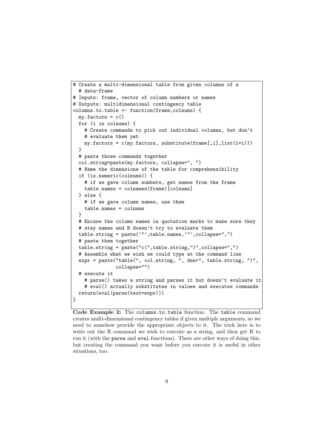
8 .meaning that inside it’s just a vector, with a fancy interface for picking out different components. I can force it back to being a vector: > as.vector(ape) [1] 34 32 2 22 11 1 0 0 and this gives me the count of each of the eight possible combinations of values for the indicator variables. Now I can invoke the entropy() function from last time: > entropy(as.vector(ape)) [1] 2.053455 So the joint entropy of the three features is just over 2 bits. Now we just need to automate this computation of the joint entropy for an arbitrary set of features. It would be nice if we could just make a vector of column numbers, v say, and then say table(nyt.frame[,v]) but unfortunately that gives a one-dimensional rather than a multi-dimensional table. (Why?) To make things work, we’ll paste together a string which would give us the commands we’d want to issue, and then have R act as though we’d typed that ourselves (Code Example 2). Let’s try this out. Sticking in all the > 0 over and over is tiresome, so I’ll just make another frame where this is done already: nyt.indicators = data.frame(class.labels=nyt.frame[,1], nyt.frame[,-1]>0) Check this on some easy cases, where we know the answers. > columns.to.table(nyt.indicators,c("class.labels")) class.labels art music 57 45 > columns.to.table(nyt.indicators,c("class.labels","art")) art class.labels FALSE TRUE art 10 47 music 37 8 > columns.to.table(nyt.indicators,c("art","painting","evening")) , , evening = FALSE painting art FALSE TRUE FALSE 34 2 TRUE 32 22 , , evening = TRUE 8 

9 .# Create a multi-dimensional table from given columns of a # data-frame # Inputs: frame, vector of column numbers or names # Outputs: multidimensional contingency table columns.to.table <- function(frame,colnums) { my.factors = c() for (i in colnums) { # Create commands to pick out individual columns, but don’t # evaluate them yet my.factors = c(my.factors, substitute(frame[,i],list(i=i))) } # paste those commands together col.string=paste(my.factors, collapse=", ") # Name the dimensions of the table for comprehensibility if (is.numeric(colnums)) { # if we gave column numbers, get names from the frame table.names = colnames(frame)[colnums] } else { # if we gave column names, use them table.names = colnums } # Encase the column names in quotation marks to make sure they # stay names and R doesn’t try to evaluate them table.string = paste(’"’,table.names,’"’,collapse=",") # paste them together table.string = paste("c(",table.string,")",collapse=",") # Assemble what we wish we could type at the command line expr = paste("table(", col.string, ", dnn=", table.string, ")", collapse="") # execute it # parse() takes a string and parses it but doesn’t evaluate it # eval() actually substitutes in values and executes commands return(eval(parse(text=expr))) } Code Example 2: The columns.to.table function. The table command creates multi-dimensional contingency tables if given multiple arguments, so we need to somehow provide the appropriate objects to it. The trick here is to write out the R command we wish to execute as a string, and then get R to run it (with the parse and eval functions). There are other ways of doing this, but creating the command you want before you execute it is useful in other situations, too. 9 

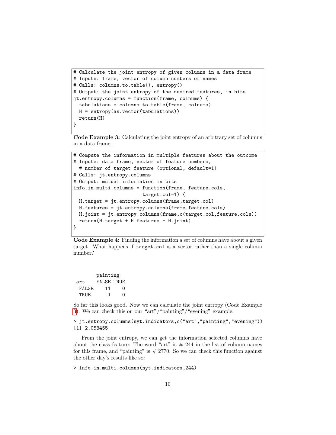
10 .# Calculate the joint entropy of given columns in a data frame # Inputs: frame, vector of column numbers or names # Calls: columns.to.table(), entropy() # Output: the joint entropy of the desired features, in bits jt.entropy.columns = function(frame, colnums) { tabulations = columns.to.table(frame, colnums) H = entropy(as.vector(tabulations)) return(H) } Code Example 3: Calculating the joint entropy of an arbitrary set of columns in a data frame. # Compute the information in multiple features about the outcome # Inputs: data frame, vector of feature numbers, # number of target feature (optional, default=1) # Calls: jt.entropy.columns # Output: mutual information in bits info.in.multi.columns = function(frame, feature.cols, target.col=1) { H.target = jt.entropy.columns(frame,target.col) H.features = jt.entropy.columns(frame,feature.cols) H.joint = jt.entropy.columns(frame,c(target.col,feature.cols)) return(H.target + H.features - H.joint) } Code Example 4: Finding the information a set of columns have about a given target. What happens if target.col is a vector rather than a single column number? painting art FALSE TRUE FALSE 11 0 TRUE 1 0 So far this looks good. Now we can calculate the joint entropy (Code Example 3). We can check this on our “art”/“painting”/“evening” example: > jt.entropy.columns(nyt.indicators,c("art","painting","evening")) [1] 2.053455 From the joint entropy, we can get the information selected columns have about the class feature: The word “art” is # 244 in the list of column names for this frame, and “painting” is # 2770. So we can check this function against the other day’s results like so: > info.in.multi.columns(nyt.indicators,244) 10 

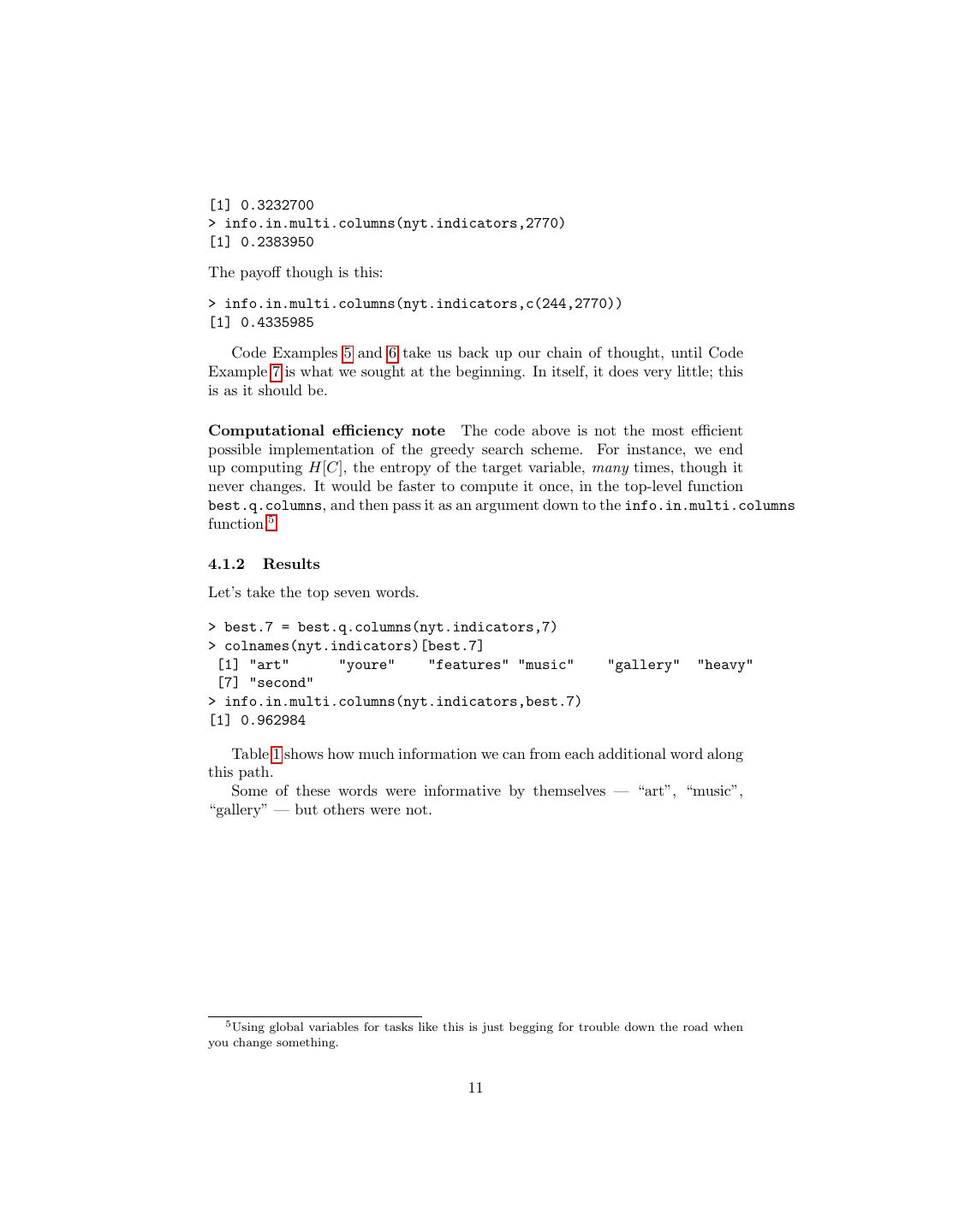
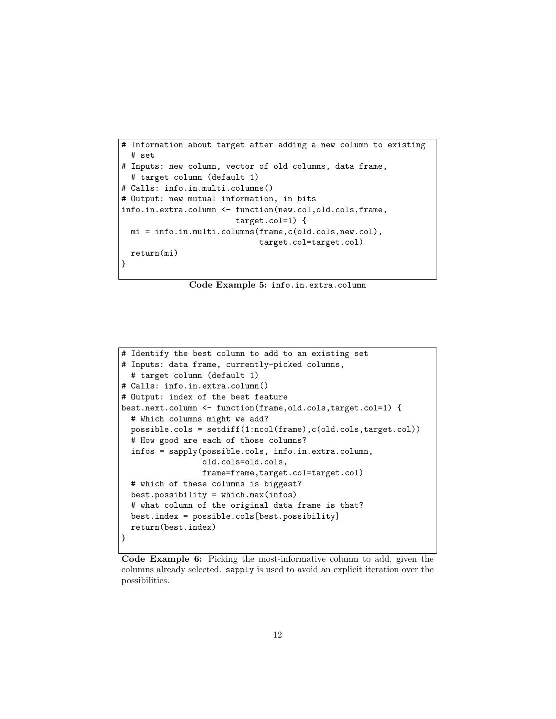
11 .[1] 0.3232700 > info.in.multi.columns(nyt.indicators,2770) [1] 0.2383950 The payoff though is this: > info.in.multi.columns(nyt.indicators,c(244,2770)) [1] 0.4335985 Code Examples 5 and 6 take us back up our chain of thought, until Code Example 7 is what we sought at the beginning. In itself, it does very little; this is as it should be. Computational efficiency note The code above is not the most efficient possible implementation of the greedy search scheme. For instance, we end up computing H[C], the entropy of the target variable, many times, though it never changes. It would be faster to compute it once, in the top-level function best.q.columns, and then pass it as an argument down to the info.in.multi.columns function.5 4.1.2 Results Let’s take the top seven words. > best.7 = best.q.columns(nyt.indicators,7) > colnames(nyt.indicators)[best.7] [1] "art" "youre" "features" "music" "gallery" "heavy" [7] "second" > info.in.multi.columns(nyt.indicators,best.7) [1] 0.962984 Table 1 shows how much information we can from each additional word along this path. Some of these words were informative by themselves — “art”, “music”, “gallery” — but others were not. 5 Using global variables for tasks like this is just begging for trouble down the road when you change something. 11 

12 .# Information about target after adding a new column to existing # set # Inputs: new column, vector of old columns, data frame, # target column (default 1) # Calls: info.in.multi.columns() # Output: new mutual information, in bits info.in.extra.column <- function(new.col,old.cols,frame, target.col=1) { mi = info.in.multi.columns(frame,c(old.cols,new.col), target.col=target.col) return(mi) } Code Example 5: info.in.extra.column # Identify the best column to add to an existing set # Inputs: data frame, currently-picked columns, # target column (default 1) # Calls: info.in.extra.column() # Output: index of the best feature best.next.column <- function(frame,old.cols,target.col=1) { # Which columns might we add? possible.cols = setdiff(1:ncol(frame),c(old.cols,target.col)) # How good are each of those columns? infos = sapply(possible.cols, info.in.extra.column, old.cols=old.cols, frame=frame,target.col=target.col) # which of these columns is biggest? best.possibility = which.max(infos) # what column of the original data frame is that? best.index = possible.cols[best.possibility] return(best.index) } Code Example 6: Picking the most-informative column to add, given the columns already selected. sapply is used to avoid an explicit iteration over the possibilities. 12 

13 .# Identify the best q columns for a given target variable # Inputs: data frame, q, target column (default 1) # Calls: best.next.column() # Output: vector of column indices best.q.columns <- function(frame,q,target.col=1) { possible.cols = setdiff(1:ncol(frame),target.col) selected.cols = c() for (k in 1:q) { new.col = best.next.column(frame,selected.cols,target.col) selected.cols=c(selected.cols,new.col) } return(selected.cols) } Code Example 7: Function for greedy selection of features by their informa- tion about a target variable. Note how almost all of the work has been passed off to other functions. word cumulative information “art” 0.32 “youre” 0.49 “features” 0.62 “music” 0.75 “gallery” 0.84 “heavy” 0.90 “second” 0.96 Table 1: The seven most informative words, as selected by the greedy search. 13 

14 .5 Sufficient Statistics and the Information Bot- tleneck For any random variable X and any function f , f (X) is another random vari- able. How does the entropy of f (X) relate to that of X? It’s easy to believe that H[X] ≥ H[f (X)] (21) After all, we can’t be more uncertain about the value of a function than about the input to the function. (Similarly, it can’t be harder to encode the function’s value.) This is in fact true, and the only way to get an equality here is if f is a one-to-one function, so it’s just, in effect, changing the label on the random variable. It’s also true that I[C; X] ≥ I[C; f (X)] (22) but now we can have equality even if f is not one-to-one. When this happens, we say that the function is sufficient for predicting C from X — it’s predictively sufficient for short, or a sufficient statistic. To mark this, we’ll write it as (X) rather than just f (X).6 Intuitively, a sufficient statistic captures all the information X has about C; everything else about X is so much extraneous detail, so how could it be of any use to us? More formally, it turns out that optimal prediction of C only needs a sufficient statistic of X, not X itself, no matter how we define “optimal”.7 All of this applies to functions of several variables as well, so if we have features X1 , . . . Xp , what we’d really like to do is find a sufficient statistic (X1 , . . . Xp ), and then forget about the original features. Unfortunately, find- ing an exactly sufficient statistic is hard, except in special cases when you make a lot of hard-to-check assumptions about the joint distribution of C and the Xi . (One which has “all the advantages of theft over honest toil” is to assume that your favorite features are sufficient; this is a key part of what’s called the method of maximum entropy.) There is however a tractable alternative for finding approximately sufficient statistics. A sufficient statistic solves the optimization problem max I[C; f (X)] (23) f ∈F where F contains all the functions of X. Let’s modify the problem: max I[C; f (X)] − βH[f (X)] (24) f ∈F 6 Of course, one-to-one functions are sufficient, but also trivial, so we’ll ignore them in what follows. 7 Even more formally: any loss function can be minimized by a decision rule which depends only on a sufficient statistic. (If you can follow that sentence, you most likely already know the result, but that’s why this is a footnote.) 14 

15 .where β is some positive number which we set. Call the solution to this problem ηβ . What happens here? Well, the objective function is indifferent between increasing I[C; f (X)] by a bit, and lowering H[f (X)] by 1/β bits. Said another way: it is willing to lose up to β bits of predictive information if doing so compresses the statistic by an extra bit. As β → 0, it becomes unwilling to lose any predictive information, and we get back a sufficient statistic. As β → ∞, we become indifferent to prediction and converge on η∞ , which is a constant function. The random variable ηβ (X) is called a bottleneck variable for predicting C from X; it’s approximately sufficient, with β indicating how big an approx- imation we’re tolerating. The method is called the information bottleneck, and the reason it’s more practical than trying to find a sufficient statistic is that there are algorithms which can solve the optimization in Eq. 24, at least if X and C are both discrete.8 This is a very cool topic — see Tishby et al. (1999) — which we may revisit if time permits. References Tishby, Naftali, Fernando C. Pereira and William Bialek (1999). “The Informa- tion Bottleneck Method.” In Proceedings of the 37th Annual Allerton Con- ference on Communication, Control and Computing (B. Hajek and R. S. Sreenivas, eds.), pp. 368–377. Urbana, Illinois: University of Illinois Press. URL http://arxiv.org/abs/physics/0004057. Verleysen, Michel, Fabrice Rossi and Damien Fran cois (2009). “Advances in Feature Selection with Mutual Information.” In Similarity-Based Clus- tering (Thomas Villmann and Michael Biehl and Barbara Hammer and Michel Verleysen, eds.), vol. 5400 of Lecture Notes in Computer Science, pp. 52–69. Berlin: Springer Verlag. URL http://arxiv.org/abs/0909.0635. doi:10.1007/978-3-642-01805-3 4. Exercises To think through, not to hand in. 1. Prove Eqs. 3 and 4. 2. What will info.in.multi.columns() do if its target.cols argument is a vector of column numbers, rather than a single column number? 8 To begin to see how this is possible, imagine that X takes on m discrete values. Then f (X) can have at most m values, too. This means that the number of possible functions of X is finite, and in principle we could evaluate the objective function of Eq. 24 on each of them. For large m the number of functions is the mth “Bell number”, and these grow very rapidly indeed — the first ten are 1, 2, 5, 15, 52, 203, 877, 4140, 21147, 115975 — so exhaustive search is out of the question, but cleverer algorithms exist. 15 

16 .3. Prove Eqs. 21 and 22. 4. Why is “youre” so informative after checking “art”? 16