信息论

1 . Finding Informative Features 36-350: Data Mining 4 September 2009 Readings: David P. Feldman, “Introduction to Information Theory”, chapter 1 (http://hornacek.coa.edu/dave/Tutorial/) Principles of Data Mining, sections 10.1, 10.2, 10.6 and 10.8 As I mentioned last time, everything we have learned how to do so far — similarity searching, nearest-neighbor and prototype classification, multidimen- sional scaling — relies on our having a vector of features or attributes for each object in data set. (The dimensionality of vector space equals the number of features.) The success of our procedures depends on our choosing good features, but I’ve said very little about how to do this. In part this is because designing good representations inevitably depends on domain knowledge. However, once we’ve picked a set of features, they’re not all necessarily equally useful, and there are some tools for quantifying that. The basic idea, remember, is that the features are the aspects of the data which show up in our representation. However, they’re not what we really care about, which is rather something we don’t, or can’t, directly represent, for instance the class of the object (is it a story about art or about music? a picture of a flower or a tiger?). We use the observable features to make a guess (formally, an inference) about the unobservable thing, like the class. Good features are ones which let us make better guesses — ones which reduce our uncertainty about the unobserved class. Good features are therefore informative, discriminative or uncertainty- reducing. This means that they need to differ across the different classes, at least statistically. I said before that the number of occurrences of the word “the” in an English document isn’t a useful feature, because it occurs about as often in all kinds of text. This means that looking at that count leaves us exactly as uncertain about which class of document we’ve seen as we were before. Similarly, the word “cystine” is going to be equally rare whether the topic is art or music, so it’s also uninformative. On the other hand, the word “rhythm” is going to be more common in stories about music than in ones about art, so counting its occurrences is going to reduce our uncertainty. The important thing is that the distribution of the feature differ across the classes. 1 

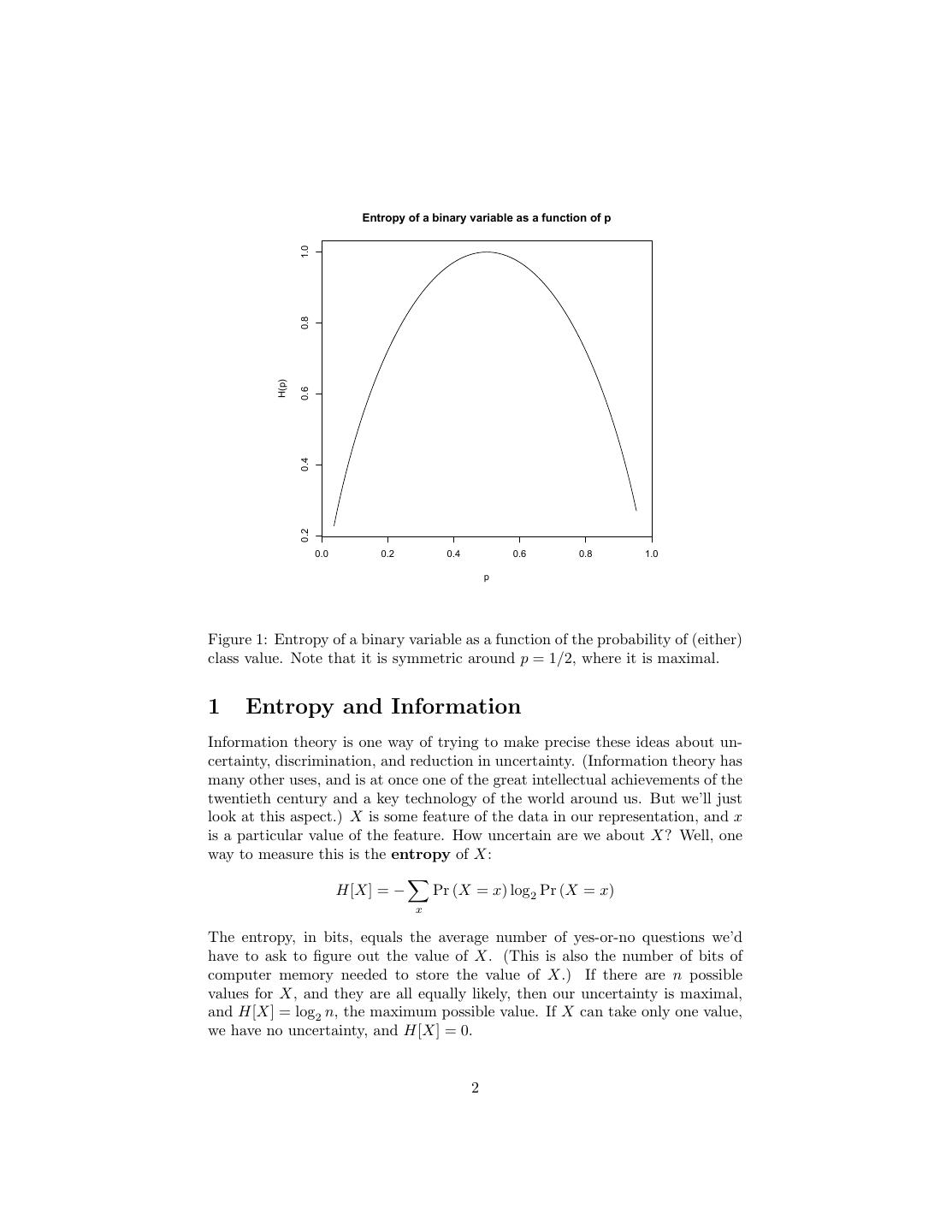
2 . Entropy of a binary variable as a function of p 1.0 0.8 H(p) 0.6 0.4 0.2 0.0 0.2 0.4 0.6 0.8 1.0 p Figure 1: Entropy of a binary variable as a function of the probability of (either) class value. Note that it is symmetric around p = 1/2, where it is maximal. 1 Entropy and Information Information theory is one way of trying to make precise these ideas about un- certainty, discrimination, and reduction in uncertainty. (Information theory has many other uses, and is at once one of the great intellectual achievements of the twentieth century and a key technology of the world around us. But we’ll just look at this aspect.) X is some feature of the data in our representation, and x is a particular value of the feature. How uncertain are we about X? Well, one way to measure this is the entropy of X: H[X] = − Pr (X = x) log2 Pr (X = x) x The entropy, in bits, equals the average number of yes-or-no questions we’d have to ask to figure out the value of X. (This is also the number of bits of computer memory needed to store the value of X.) If there are n possible values for X, and they are all equally likely, then our uncertainty is maximal, and H[X] = log2 n, the maximum possible value. If X can take only one value, we have no uncertainty, and H[X] = 0. 2 

3 . Similarly, our uncertainty about the class C, in the absence of any other information, is just the entropy of C: H[C] = − Pr (C = c) log2 Pr (C = c) c Now suppose we observe the value of the feature X. This will, in general, change our distribution for C, since we can use Bayes’s Rule: Pr (C = c, X = x) Pr (X = x|C = c) Pr (C = c|X = x) = = Pr (C = c) Pr (X = x) Pr (X = x) Pr (X = x) tells us the frequency of the value x is over the whole population. Pr (X = x|C = c) tells us the frequency of that value is when the class is c. If the two frequencies are not equal, we should change our estimate of the class, making it larger if that feature is more common in c, and making it smaller if that feature is rarer. Generally, our uncertainty about C is going to change, and be given by the conditional entropy: H[C|X = x] = − Pr (C = c|X = x) log2 Pr (C = c|X = x) c The difference in entropies, H[C]−H[C|X = x], is how much our uncertainty about C has changed, conditional on seeing X = x. This change in uncertainty is realized information: I[C; X = x] = H[C] − H[C|X = x] Notice that the realized information can be negative. For a simple example, suppose that C is “it will rain today”, and that it normally rains only one day out of seven. Then H[C] = 0.59 bits. If however we look up and see clouds (X = cloudy), and we know it rains on half of the cloudy days, H[C|X = cloudy] = 1 bit, so our uncertainty has increased by 0.41 bits. We can also look at the expected information a feature gives us about the class: I[C; X] = H[C] − H[C|X] = H[C] − Pr (X = x) H[C|X = x] x The expected information is never negative. In fact, it’s not hard to show that the only way it can even be zero is if X and C are statistically independent — if the distribution of X is the same for all classes c, Pr (X|C = c) = Pr (X) It’s also called the mutual information, because it turns out that H[C] − H[C|X] = H[X] − H[X|C]. (You might want to try to prove this to yourself, using Bayes’s rule and the definitions.) 3 

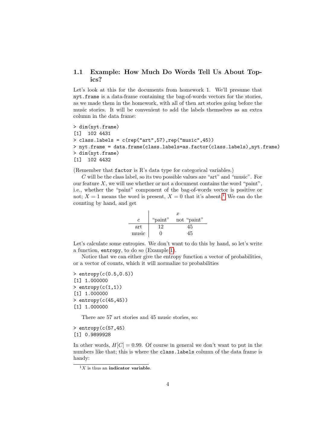
4 .1.1 Example: How Much Do Words Tell Us About Top- ics? Let’s look at this for the documents from homework 1. We’ll presume that nyt.frame is a data-frame containing the bag-of-words vectors for the stories, as we made them in the homework, with all of then art stories going before the music stories. It will be convenient to add the labels themselves as an extra column in the data frame: > dim(nyt.frame) [1] 102 4431 > class.labels = c(rep("art",57),rep("music",45)) > nyt.frame = data.frame(class.labels=as.factor(class.labels),nyt.frame) > dim(nyt.frame) [1] 102 4432 (Remember that factor is R’s data type for categorical variables.) C will be the class label, so its two possible values are “art” and “music”. For our feature X, we will use whether or not a document contains the word “paint”, i.e., whether the “paint” component of the bag-of-words vector is positive or not; X = 1 means the word is present, X = 0 that it’s absent.1 We can do the counting by hand, and get x c “paint” not “paint” art 12 45 music 0 45 Let’s calculate some entropies. We don’t want to do this by hand, so let’s write a function, entropy, to do so (Example 1). Notice that we can either give the entropy function a vector of probabilities, or a vector of counts, which it will normalize to probabilities > entropy(c(0.5,0.5)) [1] 1.000000 > entropy(c(1,1)) [1] 1.000000 > entropy(c(45,45)) [1] 1.000000 There are 57 art stories and 45 music stories, so: > entropy(c(57,45) [1] 0.9899928 In other words, H[C] = 0.99. Of course in general we don’t want to put in the numbers like that; this is where the class.labels column of the data frame is handy: 1X is thus an indicator variable. 4 

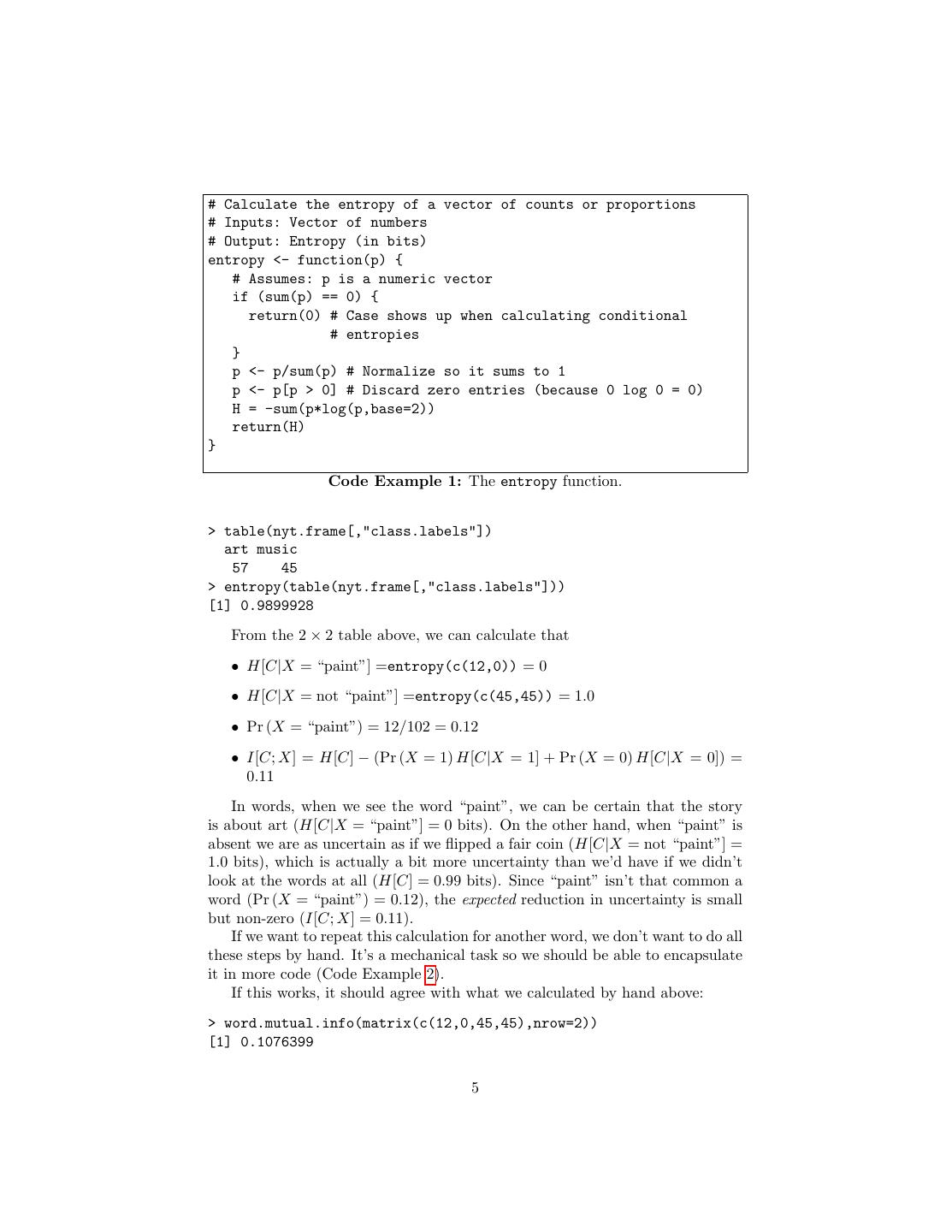
5 .# Calculate the entropy of a vector of counts or proportions # Inputs: Vector of numbers # Output: Entropy (in bits) entropy <- function(p) { # Assumes: p is a numeric vector if (sum(p) == 0) { return(0) # Case shows up when calculating conditional # entropies } p <- p/sum(p) # Normalize so it sums to 1 p <- p[p > 0] # Discard zero entries (because 0 log 0 = 0) H = -sum(p*log(p,base=2)) return(H) } Code Example 1: The entropy function. > table(nyt.frame[,"class.labels"]) art music 57 45 > entropy(table(nyt.frame[,"class.labels"])) [1] 0.9899928 From the 2 × 2 table above, we can calculate that • H[C|X = “paint”] =entropy(c(12,0)) = 0 • H[C|X = not “paint”] =entropy(c(45,45)) = 1.0 • Pr (X = “paint”) = 12/102 = 0.12 • I[C; X] = H[C] − (Pr (X = 1) H[C|X = 1] + Pr (X = 0) H[C|X = 0]) = 0.11 In words, when we see the word “paint”, we can be certain that the story is about art (H[C|X = “paint”] = 0 bits). On the other hand, when “paint” is absent we are as uncertain as if we flipped a fair coin (H[C|X = not “paint”] = 1.0 bits), which is actually a bit more uncertainty than we’d have if we didn’t look at the words at all (H[C] = 0.99 bits). Since “paint” isn’t that common a word (Pr (X = “paint”) = 0.12), the expected reduction in uncertainty is small but non-zero (I[C; X] = 0.11). If we want to repeat this calculation for another word, we don’t want to do all these steps by hand. It’s a mechanical task so we should be able to encapsulate it in more code (Code Example 2). If this works, it should agree with what we calculated by hand above: > word.mutual.info(matrix(c(12,0,45,45),nrow=2)) [1] 0.1076399 5 

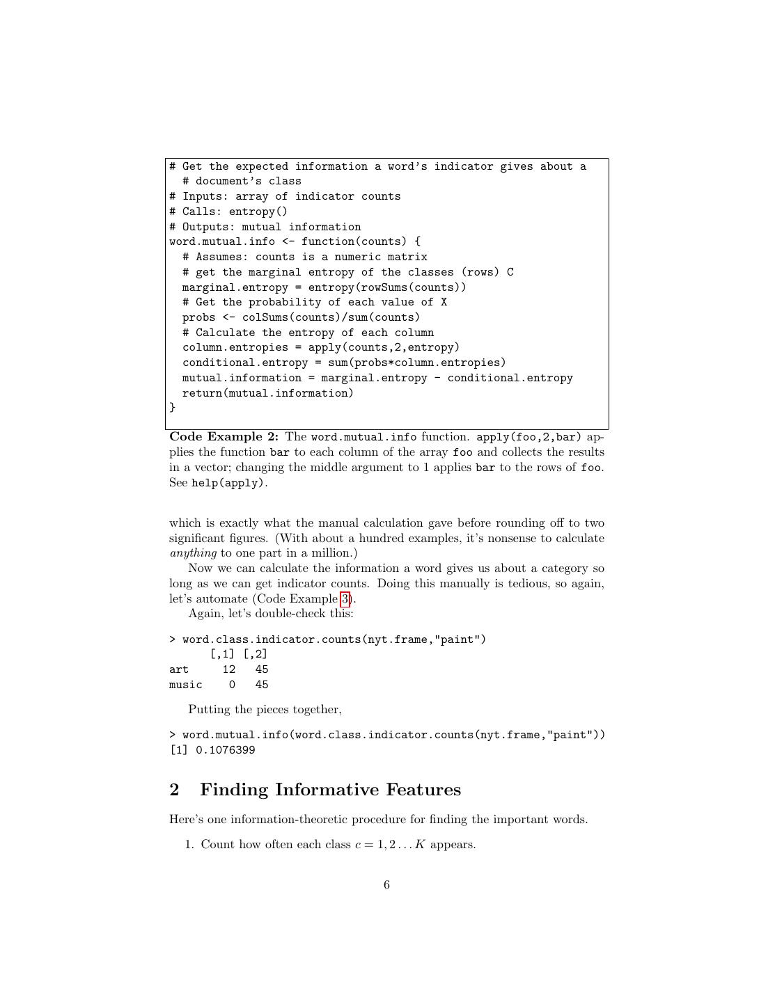
6 .# Get the expected information a word’s indicator gives about a # document’s class # Inputs: array of indicator counts # Calls: entropy() # Outputs: mutual information word.mutual.info <- function(counts) { # Assumes: counts is a numeric matrix # get the marginal entropy of the classes (rows) C marginal.entropy = entropy(rowSums(counts)) # Get the probability of each value of X probs <- colSums(counts)/sum(counts) # Calculate the entropy of each column column.entropies = apply(counts,2,entropy) conditional.entropy = sum(probs*column.entropies) mutual.information = marginal.entropy - conditional.entropy return(mutual.information) } Code Example 2: The word.mutual.info function. apply(foo,2,bar) ap- plies the function bar to each column of the array foo and collects the results in a vector; changing the middle argument to 1 applies bar to the rows of foo. See help(apply). which is exactly what the manual calculation gave before rounding off to two significant figures. (With about a hundred examples, it’s nonsense to calculate anything to one part in a million.) Now we can calculate the information a word gives us about a category so long as we can get indicator counts. Doing this manually is tedious, so again, let’s automate (Code Example 3). Again, let’s double-check this: > word.class.indicator.counts(nyt.frame,"paint") [,1] [,2] art 12 45 music 0 45 Putting the pieces together, > word.mutual.info(word.class.indicator.counts(nyt.frame,"paint")) [1] 0.1076399 2 Finding Informative Features Here’s one information-theoretic procedure for finding the important words. 1. Count how often each class c = 1, 2 . . . K appears. 6 

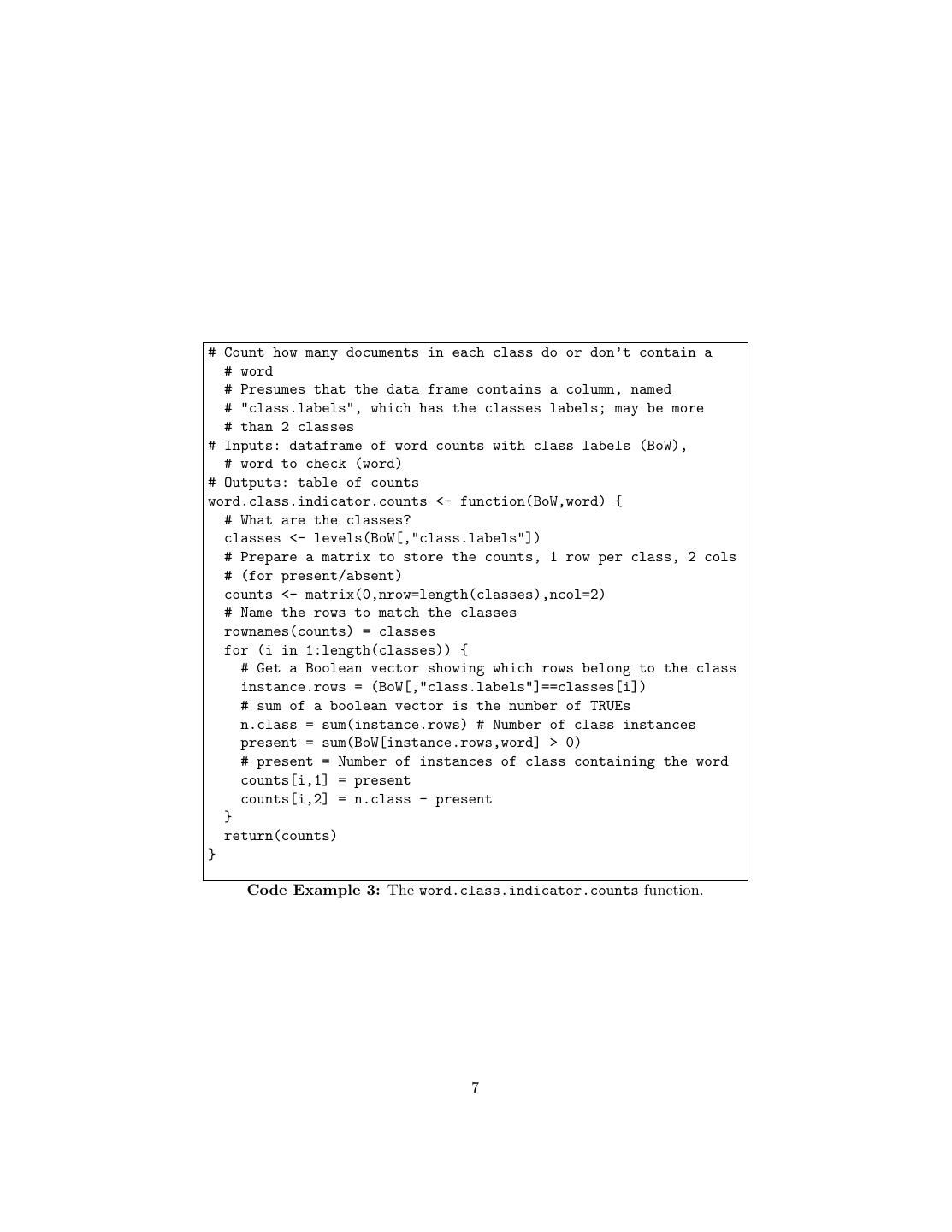
7 .# Count how many documents in each class do or don’t contain a # word # Presumes that the data frame contains a column, named # "class.labels", which has the classes labels; may be more # than 2 classes # Inputs: dataframe of word counts with class labels (BoW), # word to check (word) # Outputs: table of counts word.class.indicator.counts <- function(BoW,word) { # What are the classes? classes <- levels(BoW[,"class.labels"]) # Prepare a matrix to store the counts, 1 row per class, 2 cols # (for present/absent) counts <- matrix(0,nrow=length(classes),ncol=2) # Name the rows to match the classes rownames(counts) = classes for (i in 1:length(classes)) { # Get a Boolean vector showing which rows belong to the class instance.rows = (BoW[,"class.labels"]==classes[i]) # sum of a boolean vector is the number of TRUEs n.class = sum(instance.rows) # Number of class instances present = sum(BoW[instance.rows,word] > 0) # present = Number of instances of class containing the word counts[i,1] = present counts[i,2] = n.class - present } return(counts) } Code Example 3: The word.class.indicator.counts function. 7 

8 . 2. For each word, make the K × 2 table of classes by word indicators. 3. Compute the mutual information in each table. 4. Return the m most-informative words. This ranks words by how informative it is to see them at all in the document. We could also look at how much information we get from the number of times they appear in the document — the table we build in step two would no longer necessarily by K × 2, as the number of columns would depend on the number of different values for that word’s feature. The info.bows function (Code Example 4) does steps (1)–(3) of the ranking procedure. # Calculate realized and expected information of word indicators # for classes # Assumes: one column of the data is named "class.labels" # Inputs: data frame of word counts with class labels # Calls: word.class.indicator.counts(), word.realized.info(), # word.mutual.info() # Output: two-column matrix giving the reduction in class entropy # when a word is present, and the expected reduction from # checking the word infos.bow <- function(BoW) { lexicon <- colnames(BoW) # One of these columns will be class.labels, that’s not a # lexical item lexicon <- setdiff(lexicon,"class.labels") vocab.size = length(lexicon) word.infos <- matrix(0,nrow=vocab.size,ncol=2) # Name the rows so we know what we’re talking about rownames(word.infos) = lexicon for (i in 1:vocab.size) { counts <- word.class.indicator.counts(BoW,lexicon[i]) word.infos[i,1] = word.realized.info(counts) word.infos[i,2] = word.mutual.info(counts) } return(word.infos) } Code Example 4: The info.bows function This does two calculations for each word: how much the entropy of the class is reduced when the word is present, and how much the entropy is reduced on average by checking the word’s indicator (the mutual information). I have not given code for the function for the first calculation, word.realized.info, but you can figure it out from what I have said. 8 

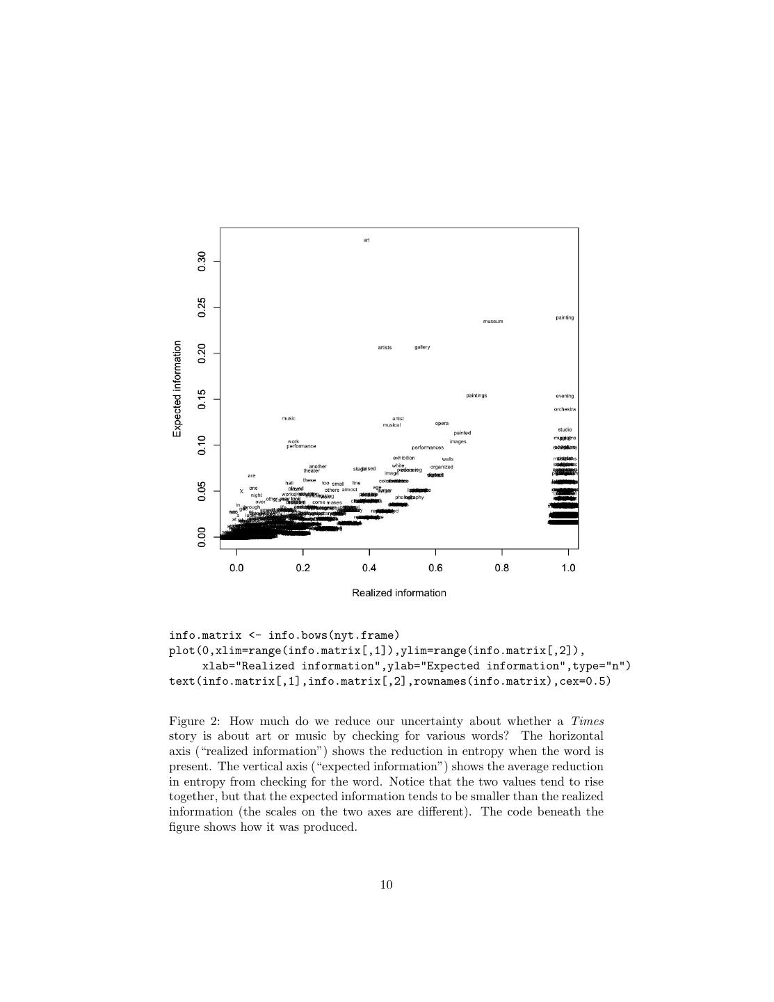
9 . I[C; X] (bits) I[C; X = 1] (bits) art 0.32 abandoned 0.99 painting 0.24 abc 0.99 museum 0.23 abroad 0.99 gallery 0.21 abstractions 0.99 artists 0.21 academic 0.99 paintings 0.15 accents 0.99 evening 0.15 accept 0.99 orchestra 0.14 acclaimed 0.99 music 0.13 accounted 0.99 artist 0.13 achievement 0.99 Table 1: Most informative words for discriminating between art and music. Left: ranked by expected information, I[C; X]. Right: ranked by realized information when the word is present, I[C; X = 1]. Table 1 shows which words’ presence or absence in a document have the most information for the art/music classification task. Figure 2 plots this for all 4431 distinct words in the data. Of course, nothing in this really hinges on our features being words; we could do the same thing for colors in a bag-of-colors representation of pictures, etc. Calculating the expected information is actually very similar to performing a χ2 test for independence. (Remember that mutual information is 0 if and only if the two variables are statistically independent.) In fact, if the sample size is large enough, the samples are IID, and the variables really are independent, then the sample mutual information has a χ2 distribution (Kullback, 1968).2 2.1 Combinations All of this is just looking at one feature at a time, so it ignores the possibility that certain combinations of features are useful, or that some features are redundant given others. We will look at this sort of interaction in the next lecture. Further Reading Information theory appeared almost fully formed in Shannon (1948), a classic paper which is remarkably readable. The best available textbook on informa- tion theory, covering its applications to coding, communications, prediction, gambling, the foundations of probability, etc., is Cover and Thomas (1991). Poundstone (2005) is a popular book about how information theory connects to gambling and the stock market; Poundstone (1984) explains how it connects to fundamental aspects of physical science, as does Wiener (1954). 2 In general, working out the bias, standard error, and sampling distribution of mutual information estimates is not easy. See, for instance, Victor (2000); Paninski (2003). 9 

10 .info.matrix <- info.bows(nyt.frame) plot(0,xlim=range(info.matrix[,1]),ylim=range(info.matrix[,2]), xlab="Realized information",ylab="Expected information",type="n") text(info.matrix[,1],info.matrix[,2],rownames(info.matrix),cex=0.5) Figure 2: How much do we reduce our uncertainty about whether a Times story is about art or music by checking for various words? The horizontal axis (“realized information”) shows the reduction in entropy when the word is present. The vertical axis (“expected information”) shows the average reduction in entropy from checking for the word. Notice that the two values tend to rise together, but that the expected information tends to be smaller than the realized information (the scales on the two axes are different). The code beneath the figure shows how it was produced. 10 

11 .References Cover, Thomas M. and Joy A. Thomas (1991). Elements of Information Theory. New York: Wiley. Kullback, Solomon (1968). Information Theory and Statistics. New York: Dover Books, 2nd edn. Paninski, Liam (2003). “Estimation of entropy and mutual information.” Neu- ral Computation, 15: 1191–1254. URL http://www.stat.columbia.edu/ ~liam/research/abstracts/info_est-nc-abs.html. Poundstone, William (1984). The Recursive Universe: Cosmic Complexity and the Limits of Scientific Knowledge. New York: William Morrow. — (2005). Fortune’s Formula: The Untold Story of the Scientific Betting Sys- tems That Beat the Casinos and Wall Street. New York: Hill and Wang. Shannon, Claude E. (1948). “A Mathematical Theory of Communication.” Bell System Technical Journal , 27: 379–423. URL http://cm.bell-labs.com/ cm/ms/what/shannonday/paper.html. Reprinted in Shannon and Weaver (1963). Shannon, Claude E. and Warren Weaver (1963). The Mathematical Theory of Communication. Urbana, Illinois: University of Illinois Press. Victor, Jonathan D. (2000). “Asymptotic Bias in Information Estimates and the Exponential (Bell) Polynomials.” Neural Computation, 12: 2797–2804. Wiener, Norbert (1954). The Human Use of Human Beings: Cybernetics and Society. Garden City, New York: Doubleday, 2nd edn. Republished London: Free Association Books, 1989; first ed. Boston: Houghton Mifflin, 1950. 11 

12 .Exercises These are for you to think about, rather than to hand in. 1. How would you reproduce Figure 1? 2. Looking at Figure 2, why does expected information tend to generally increase with realized information? 3. Why does expected information tend to be smaller than realized informa- tion? 4. Why are so many words vertically aligned at the right edge of the plot? 5. Write word.realized.info. 6. What code would you have to change to calculate the information the number of appearances of a word gives you about the class? 7. Read help(order). How would you reproduce Table 1? 12