Density Estimation

1 . Estimating Distributions and Densities 36-350, Data Mining, Fall 2009 23 November 2009 Contents 1 “The Fundamental Theorem of Statistics” 2 2 Error for Density Estimates 3 3 Kernel Density Estimates 4 3.1 More on the Expected Log-Likelihood Ratio . . . . . . . . . . . . 5 4 Other Approaches 7 For most of you, making a histogram was probably one of the first things you learned how to do in baby stats (if not before). This is a simple way of estimating a distribution: we split the sample space up into bins, count how many samples fall into each bin, and then divide the counts by the total number of samples. If we hold the bins fixed and take more and more data, then by the law of large numbers we anticipate that the relative frequency for each bin will converge on the bin’s probability. So far so good. But one of the things you learned in baby stats was also to work with probability density functions, not just probability mass functions. Where do we get pdfs? Well, one thing we could do is to take our histogram estimate, and then say that the probability density is uniform within each bin. This gives us a piecewise-constant estimate of the density. Unfortunately, this isn’t going to work — isn’t going to converge on the true pdf — unless we can shrink the bins of the histogram as we get more and more data. To see this, think about estimating the pdf when the data comes from any of the standard distributions, like an exponential or a Gaussian. We can approximate the true pdf f (x) to arbitrary accuracy by a piecewise-constant density (indeed, that’s what all our plotting code does!), but, for a fixed set of bins, we can only come so close but no closer to the true, continuous density. This reminds us of our old friend the bias-variance trade-off, and in fact that’s correct. If we use a large number of very small bins, the minimum bias in our estimate of any density becomes small, but the variance in our estimates grows. (Why does variance increase?) To make some use of this insight, though, there are some things we need to establish first. • Is learning the whole distribution non-parametrically even feasible? 1 

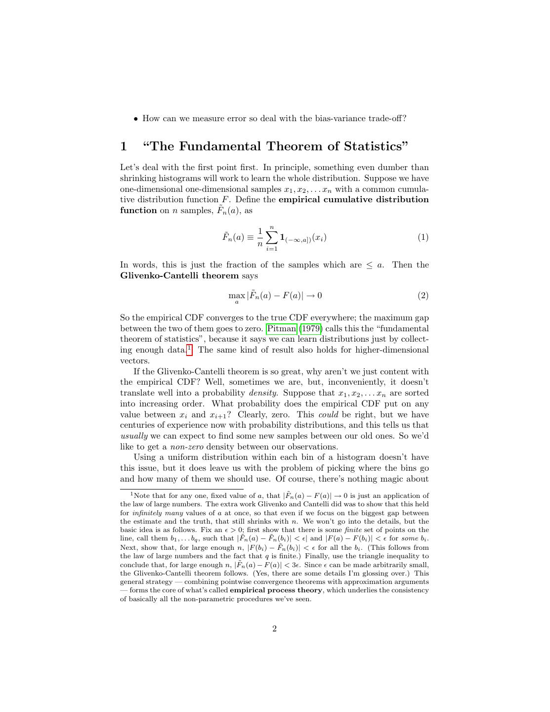
2 . • How can we measure error so deal with the bias-variance trade-off? 1 “The Fundamental Theorem of Statistics” Let’s deal with the first point first. In principle, something even dumber than shrinking histograms will work to learn the whole distribution. Suppose we have one-dimensional one-dimensional samples x1 , x2 , . . . xn with a common cumula- tive distribution function F . Define the empirical cumulative distribution function on n samples, F˜n (a), as n 1 F˜n (a) ≡ 1(−∞,a]) (xi ) (1) n i=1 In words, this is just the fraction of the samples which are ≤ a. Then the Glivenko-Cantelli theorem says max |F˜n (a) − F (a)| → 0 (2) a So the empirical CDF converges to the true CDF everywhere; the maximum gap between the two of them goes to zero. Pitman (1979) calls this the “fundamental theorem of statistics”, because it says we can learn distributions just by collect- ing enough data.1 The same kind of result also holds for higher-dimensional vectors. If the Glivenko-Cantelli theorem is so great, why aren’t we just content with the empirical CDF? Well, sometimes we are, but, inconveniently, it doesn’t translate well into a probability density. Suppose that x1 , x2 , . . . xn are sorted into increasing order. What probability does the empirical CDF put on any value between xi and xi+1 ? Clearly, zero. This could be right, but we have centuries of experience now with probability distributions, and this tells us that usually we can expect to find some new samples between our old ones. So we’d like to get a non-zero density between our observations. Using a uniform distribution within each bin of a histogram doesn’t have this issue, but it does leave us with the problem of picking where the bins go and how many of them we should use. Of course, there’s nothing magic about 1 Note that for any one, fixed value of a, that |F ˜n (a) − F (a)| → 0 is just an application of the law of large numbers. The extra work Glivenko and Cantelli did was to show that this held for infinitely many values of a at once, so that even if we focus on the biggest gap between the estimate and the truth, that still shrinks with n. We won’t go into the details, but the basic idea is as follows. Fix an > 0; first show that there is some finite set of points on the line, call them b1 , . . . bq , such that |F˜n (a) − F˜n (bi )| < | and |F (a) − F (bi )| < for some bi . Next, show that, for large enough n, |F (bi ) − F˜n (bi )| < for all the bi . (This follows from the law of large numbers and the fact that q is finite.) Finally, use the triangle inequality to conclude that, for large enough n, |F˜n (a) − F (a)| < 3 . Since can be made arbitrarily small, the Glivenko-Cantelli theorem follows. (Yes, there are some details I’m glossing over.) This general strategy — combining pointwise convergence theorems with approximation arguments — forms the core of what’s called empirical process theory, which underlies the consistency of basically all the non-parametric procedures we’ve seen. 2 

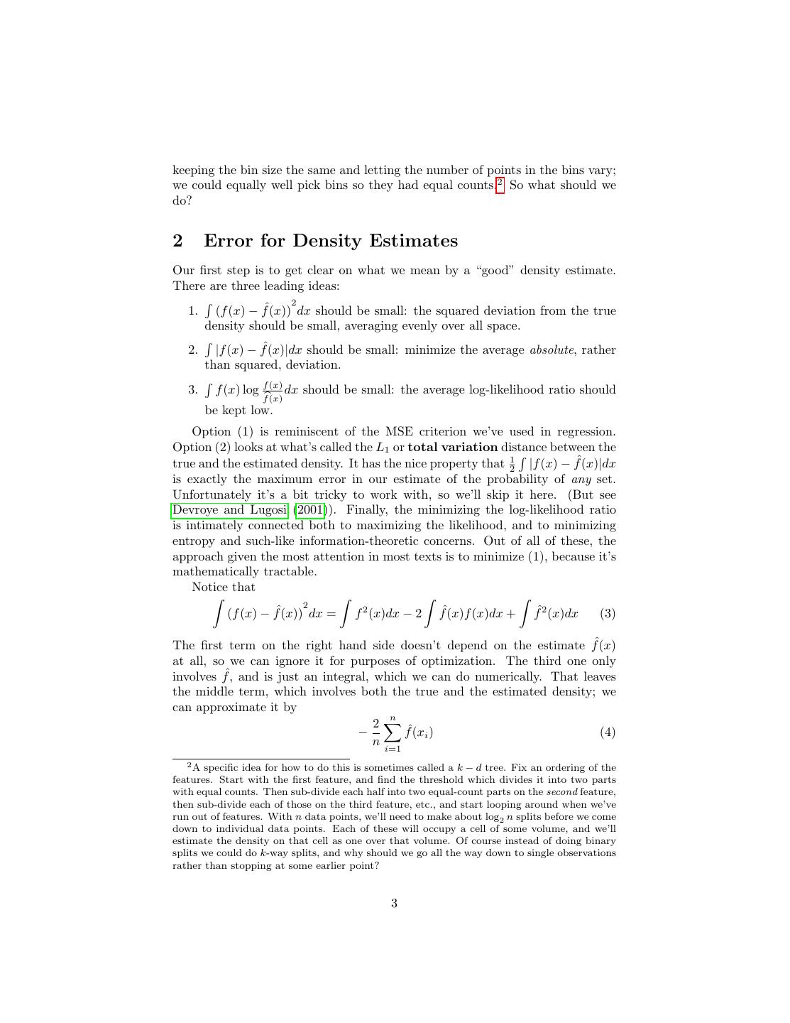
3 .keeping the bin size the same and letting the number of points in the bins vary; we could equally well pick bins so they had equal counts.2 So what should we do? 2 Error for Density Estimates Our first step is to get clear on what we mean by a “good” density estimate. There are three leading ideas: 2 1. (f (x) − fˆ(x)) dx should be small: the squared deviation from the true density should be small, averaging evenly over all space. 2. |f (x) − fˆ(x)|dx should be small: minimize the average absolute, rather than squared, deviation. f (x) 3. f (x) log dx should be small: the average log-likelihood ratio should f (x) be kept low. Option (1) is reminiscent of the MSE criterion we’ve used in regression. Option (2) looks at what’s called the L1 or total variation distance between the true and the estimated density. It has the nice property that 12 |f (x) − fˆ(x)|dx is exactly the maximum error in our estimate of the probability of any set. Unfortunately it’s a bit tricky to work with, so we’ll skip it here. (But see Devroye and Lugosi (2001)). Finally, the minimizing the log-likelihood ratio is intimately connected both to maximizing the likelihood, and to minimizing entropy and such-like information-theoretic concerns. Out of all of these, the approach given the most attention in most texts is to minimize (1), because it’s mathematically tractable. Notice that 2 (f (x) − fˆ(x)) dx = f 2 (x)dx − 2 fˆ(x)f (x)dx + fˆ2 (x)dx (3) The first term on the right hand side doesn’t depend on the estimate fˆ(x) at all, so we can ignore it for purposes of optimization. The third one only involves fˆ, and is just an integral, which we can do numerically. That leaves the middle term, which involves both the true and the estimated density; we can approximate it by n 2 − fˆ(xi ) (4) n i=1 2 A specific idea for how to do this is sometimes called a k − d tree. Fix an ordering of the features. Start with the first feature, and find the threshold which divides it into two parts with equal counts. Then sub-divide each half into two equal-count parts on the second feature, then sub-divide each of those on the third feature, etc., and start looping around when we’ve run out of features. With n data points, we’ll need to make about log2 n splits before we come down to individual data points. Each of these will occupy a cell of some volume, and we’ll estimate the density on that cell as one over that volume. Of course instead of doing binary splits we could do k-way splits, and why should we go all the way down to single observations rather than stopping at some earlier point? 3 

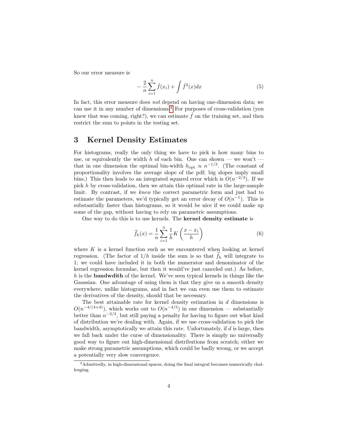
4 .So our error measure is n 2 − fˆ(xi ) + fˆ2 (x)dx (5) n i=1 In fact, this error measure does not depend on having one-dimension data; we can use it in any number of dimensions.3 For purposes of cross-validation (you knew that was coming, right?), we can estimate fˆ on the training set, and then restrict the sum to points in the testing set. 3 Kernel Density Estimates For histograms, really the only thing we have to pick is how many bins to use, or equivalently the width h of each bin. One can shown — we won’t — that in one dimension the optimal bin-width hopt ∝ n−1/3 . (The constant of proportionality involves the average slope of the pdf; big slopes imply small bins.) This then leads to an integrated squared error which is O(n−2/3 ). If we pick h by cross-validation, then we attain this optimal rate in the large-sample limit. By contrast, if we knew the correct parametric form and just had to estimate the parameters, we’d typically get an error decay of O(n−1 ). This is substantially faster than histograms, so it would be nice if we could make up some of the gap, without having to rely on parametric assumptions. One way to do this is to use kernels. The kernel density estimate is n 1 1 x − xi fh (x) = K (6) n i=1 h h where K is a kernel function such as we encountered when looking at kernel regression. (The factor of 1/h inside the sum is so that fh will integrate to 1; we could have included it in both the numerator and denominator of the kernel regression formulae, but then it would’ve just canceled out.) As before, h is the bandwdith of the kernel. We’ve seen typical kernels in things like the Gaussian. One advantage of using them is that they give us a smooth density everywhere, unlike histograms, and in fact we can even use them to estimate the derivatives of the density, should that be necessary. The best attainable rate for kernel density estimation in d dimensions is O(n−4/(4+d) ), which works out to O(n−4/5 ) in one dimension — substantially better than n−2/3 , but still paying a penalty for having to figure out what kind of distribution we’re dealing with. Again, if we use cross-validation to pick the bandwidth, asymptotically we attain this rate. Unfortunately, if d is large, then we fall back under the curse of dimensionality. There is simply no universally good way to figure out high-dimensional distributions from scratch; either we make strong parametric assumptions, which could be badly wrong, or we accept a potentially very slow convergence. 3 Admittedly, in high-dimensional spaces, doing the final integral becomes numerically chal- lenging. 4 

5 . As an alternative to cross-validation, or at least a starting point, one can show that the optimal bandwidth for using a Gaussian kernel to estimate a Gaussian distribution is 1.06σ/n1/5 , with σ being the standard deviation of the Gaussian. This is sometimes called the Gaussian reference rule or the rule- of-thumb bandwidth. When you call density in R, this is basically what it does. One can employ the plug-in method here: given an initial bandwidth (as from the rule-of-thumb), get a crude estimate of the density, plug that in to the optimal bandwidth formulas, use that to re-estimate the density, etc. In addition to estimating marginal and joint densities, we will often want to get conditional densities. The most straightforward way to get the density of Y given X, fY |X (y|x), is fX,Y (x, y) fY |X (y|x) = (7) fX (x) i.e., to estimate the joint and marginal densities and divide one by the other. The np package implements this, including a sensible treatment of the case where some of the components of x are categorical or ordered variables, in its npcends function (Hayfield and Racine, 2008). (npudens estimates unconditional joint distributions.) One trick — exploited by np — is worth remarking on. Say that x = (x1 , x2 ), and that y is independent of x2 given x1 . Then the best bandwidth to use for x2 in estimating fY |X1 ,X2 (y|x1 , x2 ) is not the bandwidth one would use when estimating fX2 (x2 ). Rather, we don’t care about the density of x2 , so we’d like to set its bandwidth to infinity and ignore it. Cross-validation, remarkably enough, will tend to do this (Hall et al., 2004). Sampling from a kernel density estimate There are times when one wants to draw a random sample from the estimated distribution. This is easy with kernel density estimates, because each kernel is itself a probability density, gen- erally a very tractable one. The general pattern goes as follows. Suppose the kernel is Gaussian, that we have scalar observations x1 , x2 , . . . xn , and the se- lected bandwidth is h. Then we pick an integer uniformly at random from 1 to n, and invoke rnorm(1,x[i],h).4 Using a different kernel, we’d just need to use the random number generator function for the corresponding distribution. 3.1 More on the Expected Log-Likelihood Ratio f (x) I want to say just a bit more about the expected log-likelihood ratio f (x) log dx. f (x) More formally, this is called the Kullback-Leibler divergence or relative entropy of f from f , and is also written D(f f ). Let’s expand the log ratio: D(f f ) = − f (x) log f (x)dx + f (x) log f (x)dx (8) 4 In fact, if we want to draw a sample of size q, rnorm(q,sample(x,q,replace=TRUE),h) will work in R — it’s important hough that sampling be done with replacement (the default is to not replace). 5 

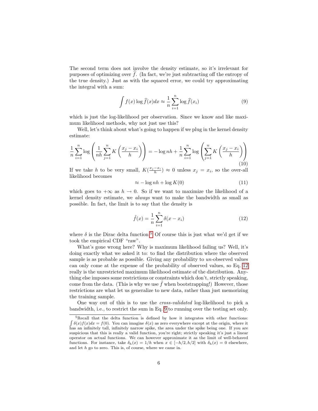
6 .The second term does not involve the density estimate, so it’s irrelevant for purposes of optimizing over f . (In fact, we’re just subtracting off the entropy of the true density.) Just as with the squared error, we could try approximating the integral with a sum: n 1 f (x) log f (x)dx ≈ log f (xi ) (9) n i=1 which is just the log-likelihood per observation. Since we know and like maxi- mum likelihood methods, why not just use this? Well, let’s think about what’s going to happen if we plug in the kernel density estimate:     n n n n 1 1 xj − xi  1 xj − xi  log  K = − log nh + log  K n i=1 nh j=1 h n i=1 j=1 h (10) x −x If we take h to be very small, K( j h i ) ≈ 0 unless xj = xi , so the over-all likelihood becomes ≈ − log nh + log K(0) (11) which goes to +∞ as h → 0. So if we want to maximize the likelihood of a kernel density estimate, we always want to make the bandwidth as small as possible. In fact, the limit is to say that the density is n 1 f˜(x) = δ(x − xi ) (12) n i=1 where δ is the Dirac delta function.5 Of course this is just what we’d get if we took the empirical CDF “raw”. What’s gone wrong here? Why is maximum likelihood failing us? Well, it’s doing exactly what we asked it to: to find the distribution where the observed sample is as probable as possible. Giving any probability to un-observed values can only come at the expense of the probability of observed values, so Eq. 12 really is the unrestricted maximum likelihood estimate of the distribution. Any- thing else imposes some restrictions or constraints which don’t, strictly speaking, come from the data. (This is why we use f˜ when bootstrapping!) However, those restrictions are what let us generalize to new data, rather than just memorizing the training sample. One way out of this is to use the cross-validated log-likelihood to pick a bandwidth, i.e., to restrict the sum in Eq. 9 to running over the testing set only. 5 Recall that the delta function is defined by how it integrates with other functions: δ(x)f (x)dx = f (0). You can imagine δ(x) as zero everywhere except at the origin, where it has an infinitely tall, infinitely narrow spike, the area under the spike being one. If you are suspicious that this is really a valid function, you’re right; strictly speaking it’s just a linear operator on actual functions. We can however approximate it as the limit of well-behaved functions. For instance, take δh (x) = 1/h when x ∈ [−h/2, h/2] with δh (x) = 0 elsewhere, and let h go to zero. This is, of course, where we came in. 6 

7 .This way, very small bandwidths don’t get an unfair advantage for concentrating around the training set. (If the test points are in fact all very close to the training points, then small bandwidths get a fair advantage.) This is in fact the default procedure in the np package, through the bwmethod option ("cv.ml" vs. "cv.ls"). 4 Other Approaches Of course, histograms and kernels aren’t the only possible way of estimating densities. One can try the local polynomial trick, series expansions, splines, etc. For some of these, one wants to avoid the embarrassment of negative probability density estimates (what would those even mean?), and so one works with, say, the log density. References Devroye, Luc and G´ abor Lugosi (2001). Combinatorial Methods in Density Estimation. Berlin: Springer-Verlag. Hall, Peter, Jeff Racine and Qi Li (2004). “Cross-Validation and the Estimation of Conditional Probability Densities.” Journal of the American Statistical Association, 99: 1015–1026. URL http://www.ssc.wisc.edu/~bhansen/ workshop/QiLi.pdf. Hayfield, Tristen and Jeffrey S. Racine (2008). “Nonparametric Econometrics: The np Package.” Journal of Statistical Software, 27(5): 1–32. URL http: //www.jstatsoft.org/v27/i05. Pitman, E. J. G. (1979). Some Basic Theory for Statistical Inference. London: Chapman and Hall. 7