Geometry of linear classifiers.

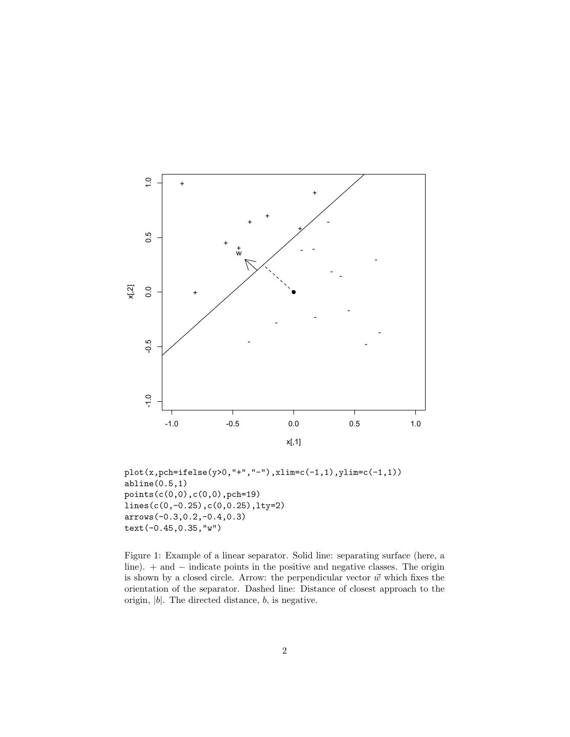
1 . Linear Classifiers and the Perceptron Algorithm 36-350, Data Mining, Fall 2009 16 November 2009 Contents 1 Linear Classifiers 1 2 The Perceptron Algorithm 3 1 Linear Classifiers Notation: x is a vector of real-valued numerical input features; we’ll say there are p of them. The response is a binary class Y ; it will simplify the book-keeping to say that the two classes are +1 and −1. In linear classification, we seek to divide the two classes by a linear separator in the feature space. If p = 2, the separator is a line, if p = 3 it’s a plane, and in general it’s a (p − 1)-dimensional hyper-plane in a p-dimensional space; I will say “plane” without loss of generality. We can specify the orientation of a plane by a vector w in the direction perpendicular to it.1 There are infinitely many parallel planes with the same orientation; we need to pick out one of them, which we can do by saying how close it comes to the origin. We’d like a formula to express the idea that points on one side of the plane belong to one class, and those on the other side belong to a different class. We can do this as: y(x, b, w) = sgn b + x · w (1) p where, as a reminder, x · w = j=1 xj wj . The sign function sgn is normally defined to return +1 if its argument is > 0, −1 if its argument is < 0, and 0 if its argument is zero. We will silently re-define it so that it never gives zero (which would be classless); but it doesn’t matter how, so after tossing a coin I say that it gives +1 if its argument is non-negative. Remember that if w is a unit vector, then x · w is the projection of x on to that direction, so this is in fact checking whether x is on the positive side of the separating plane or not. 1 Of course there are two such “normal” vectors for any plane, pointing in opposite direc- tions. As we’ll see in a moment, which vector we pick determines which side of the plane is “+” and which is “-”. 1 

2 . 1.0 + + + + - + 0.5 + + - - w - - - x[,2] 0.0 + - - - - - - -0.5 -1.0 -1.0 -0.5 0.0 0.5 1.0 x[,1] plot(x,pch=ifelse(y>0,"+","-"),xlim=c(-1,1),ylim=c(-1,1)) abline(0.5,1) points(c(0,0),c(0,0),pch=19) lines(c(0,-0.25),c(0,0.25),lty=2) arrows(-0.3,0.2,-0.4,0.3) text(-0.45,0.35,"w") Figure 1: Example of a linear separator. Solid line: separating surface (here, a line). + and − indicate points in the positive and negative classes. The origin is shown by a closed circle. Arrow: the perpendicular vector w which fixes the orientation of the separator. Dashed line: Distance of closest approach to the origin, |b|. The directed distance, b, is negative. 2 

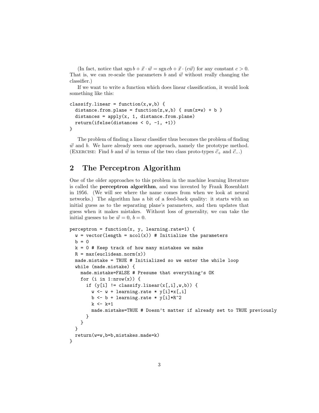
3 . (In fact, notice that sgn b + x · w = sgn cb + x · (cw) for any constant c > 0. That is, we can re-scale the parameters b and w without really changing the classifier.) If we want to write a function which does linear classification, it would look something like this: classify.linear = function(x,w,b) { distance.from.plane = function(z,w,b) { sum(z*w) + b } distances = apply(x, 1, distance.from.plane) return(ifelse(distances < 0, -1, +1)) } The problem of finding a linear classifier thus becomes the problem of finding w and b. We have already seen one approach, namely the prototype method. (Exercise: Find b and w in terms of the two class proto-types c+ and c− .) 2 The Perceptron Algorithm One of the older approaches to this problem in the machine learning literature is called the perceptron algorithm, and was invented by Frank Rosenblatt in 1956. (We will see where the name comes from when we look at neural networks.) The algorithm has a bit of a feed-back quality: it starts with an initial guess as to the separating plane’s parameters, and then updates that guess when it makes mistakes. Without loss of generality, we can take the initial guesses to be w = 0, b = 0. perceptron = function(x, y, learning.rate=1) { w = vector(length = ncol(x)) # Initialize the parameters b = 0 k = 0 # Keep track of how many mistakes we make R = max(euclidean.norm(x)) made.mistake = TRUE # Initialized so we enter the while loop while (made.mistake) { made.mistake=FALSE # Presume that everything’s OK for (i in 1:nrow(x)) { if (y[i] != classify.linear(x[,i],w,b)) { w <- w + learning.rate * y[i]*x[,i] b <- b + learning.rate * y[i]*R^2 k <- k+1 made.mistake=TRUE # Doesn’t matter if already set to TRUE previously } } } return(w=w,b=b,mistakes.made=k) } 3 

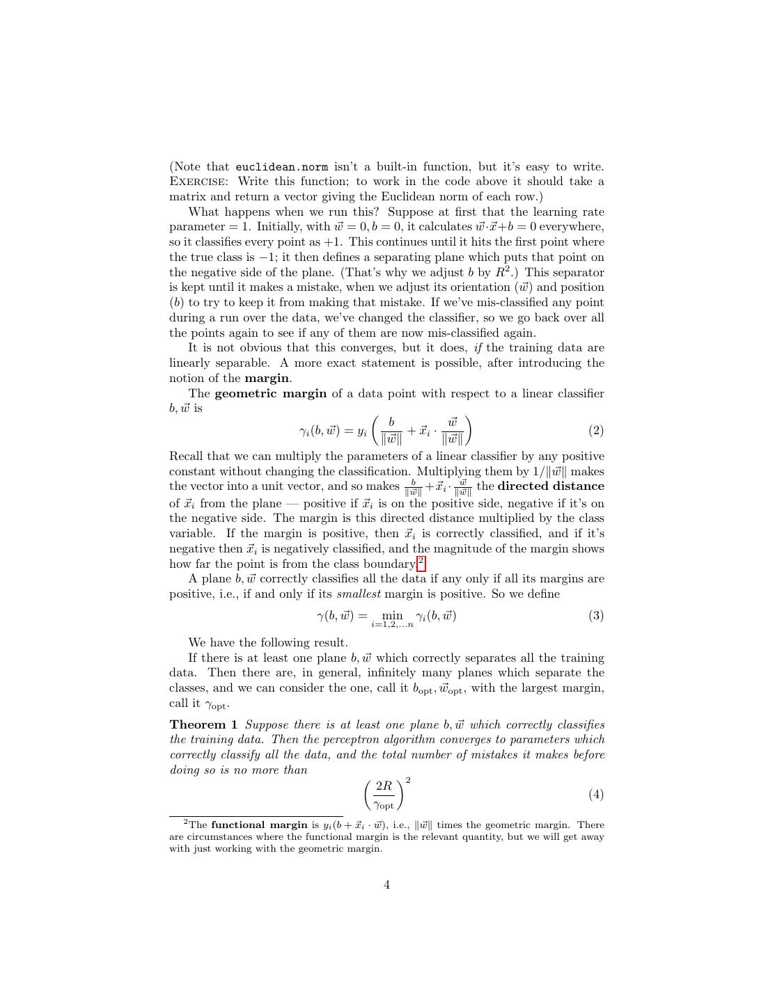
4 .(Note that euclidean.norm isn’t a built-in function, but it’s easy to write. Exercise: Write this function; to work in the code above it should take a matrix and return a vector giving the Euclidean norm of each row.) What happens when we run this? Suppose at first that the learning rate parameter = 1. Initially, with w = 0, b = 0, it calculates w·x+b = 0 everywhere, so it classifies every point as +1. This continues until it hits the first point where the true class is −1; it then defines a separating plane which puts that point on the negative side of the plane. (That’s why we adjust b by R2 .) This separator is kept until it makes a mistake, when we adjust its orientation (w) and position (b) to try to keep it from making that mistake. If we’ve mis-classified any point during a run over the data, we’ve changed the classifier, so we go back over all the points again to see if any of them are now mis-classified again. It is not obvious that this converges, but it does, if the training data are linearly separable. A more exact statement is possible, after introducing the notion of the margin. The geometric margin of a data point with respect to a linear classifier b, w is b w γi (b, w) = yi + xi · (2) w w Recall that we can multiply the parameters of a linear classifier by any positive constant without changing the classification. Multiplying them by 1/ w makes the vector into a unit vector, and so makes wb +xi · w w the directed distance of xi from the plane — positive if xi is on the positive side, negative if it’s on the negative side. The margin is this directed distance multiplied by the class variable. If the margin is positive, then xi is correctly classified, and if it’s negative then xi is negatively classified, and the magnitude of the margin shows how far the point is from the class boundary.2 A plane b, w correctly classifies all the data if any only if all its margins are positive, i.e., if and only if its smallest margin is positive. So we define γ(b, w) = min γi (b, w) (3) i=1,2,...n We have the following result. If there is at least one plane b, w which correctly separates all the training data. Then there are, in general, infinitely many planes which separate the classes, and we can consider the one, call it bopt , wopt , with the largest margin, call it γopt . Theorem 1 Suppose there is at least one plane b, w which correctly classifies the training data. Then the perceptron algorithm converges to parameters which correctly classify all the data, and the total number of mistakes it makes before doing so is no more than 2 2R (4) γopt 2 The functional margin is yi (b + xi · w), i.e., w times the geometric margin. There are circumstances where the functional margin is the relevant quantity, but we will get away with just working with the geometric margin. 4 

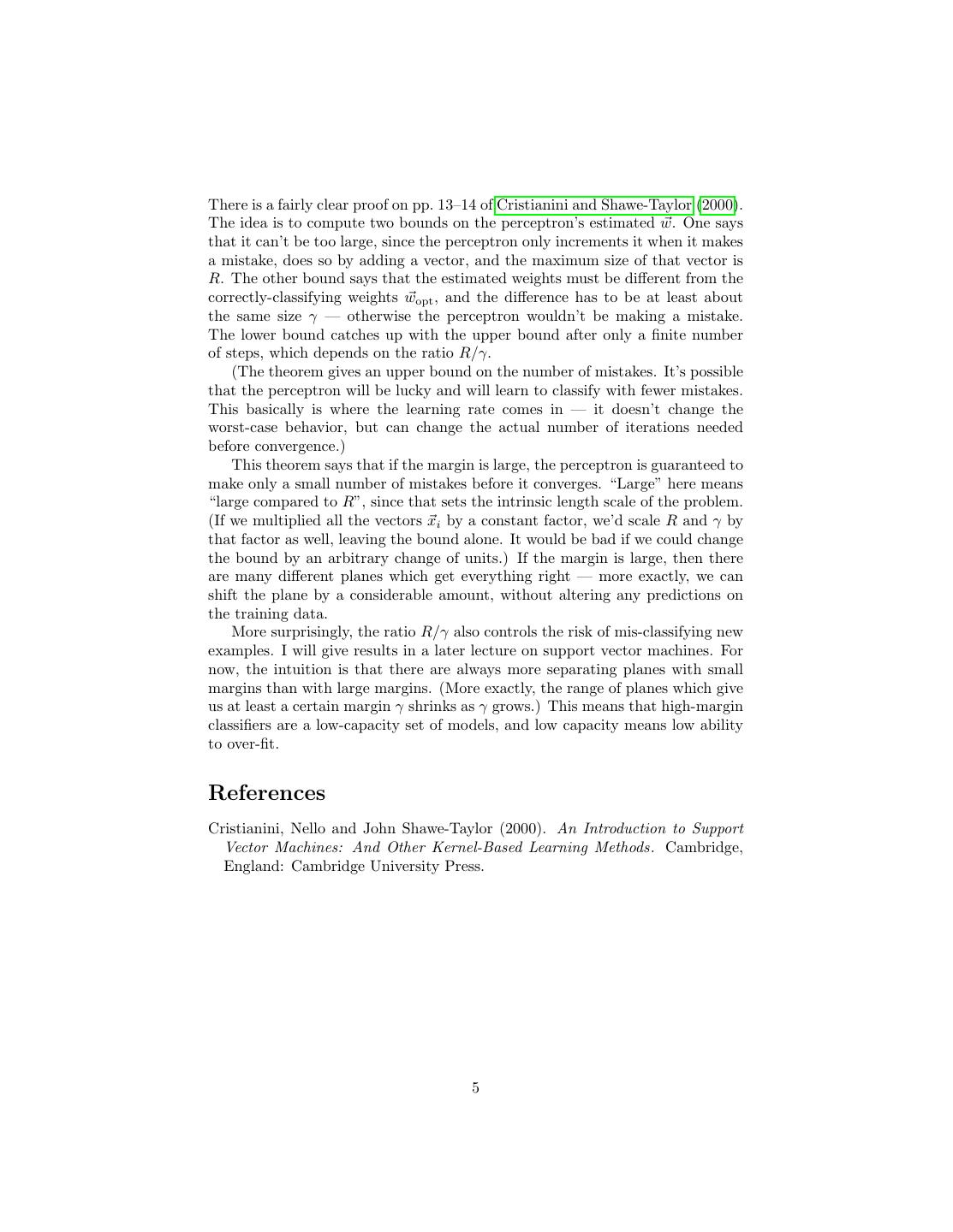
5 .There is a fairly clear proof on pp. 13–14 of Cristianini and Shawe-Taylor (2000). The idea is to compute two bounds on the perceptron’s estimated w. One says that it can’t be too large, since the perceptron only increments it when it makes a mistake, does so by adding a vector, and the maximum size of that vector is R. The other bound says that the estimated weights must be different from the correctly-classifying weights wopt , and the difference has to be at least about the same size γ — otherwise the perceptron wouldn’t be making a mistake. The lower bound catches up with the upper bound after only a finite number of steps, which depends on the ratio R/γ. (The theorem gives an upper bound on the number of mistakes. It’s possible that the perceptron will be lucky and will learn to classify with fewer mistakes. This basically is where the learning rate comes in — it doesn’t change the worst-case behavior, but can change the actual number of iterations needed before convergence.) This theorem says that if the margin is large, the perceptron is guaranteed to make only a small number of mistakes before it converges. “Large” here means “large compared to R”, since that sets the intrinsic length scale of the problem. (If we multiplied all the vectors xi by a constant factor, we’d scale R and γ by that factor as well, leaving the bound alone. It would be bad if we could change the bound by an arbitrary change of units.) If the margin is large, then there are many different planes which get everything right — more exactly, we can shift the plane by a considerable amount, without altering any predictions on the training data. More surprisingly, the ratio R/γ also controls the risk of mis-classifying new examples. I will give results in a later lecture on support vector machines. For now, the intuition is that there are always more separating planes with small margins than with large margins. (More exactly, the range of planes which give us at least a certain margin γ shrinks as γ grows.) This means that high-margin classifiers are a low-capacity set of models, and low capacity means low ability to over-fit. References Cristianini, Nello and John Shawe-Taylor (2000). An Introduction to Support Vector Machines: And Other Kernel-Based Learning Methods. Cambridge, England: Cambridge University Press. 5