Evaluating Predictive Models

1 . Evaluating Predictive Models 36-350, Data Mining 26 and 28 October 2009 Readings: Principles of Data Mining, chapter 7; Berk, chapter 2. Contents 1 Errors, In and Out of Sample 1 2 Some Examples: Over-Fitting and Under-Fitting 4 3 Model Selection and Capacity Control 16 3.1 Big Data . . . . . . . . . . . . . . . . . . . . . . . . . . . . . . . . 16 3.2 Penalization . . . . . . . . . . . . . . . . . . . . . . . . . . . . . . 17 3.3 From Penalties to Constraints; the Method of Sieves . . . . . . . 18 3.4 Capacity Control . . . . . . . . . . . . . . . . . . . . . . . . . . . 19 3.5 Cross-Validation . . . . . . . . . . . . . . . . . . . . . . . . . . . 20 3.6 Why Chose? . . . . . . . . . . . . . . . . . . . . . . . . . . . . . . 21 4 Warnings 21 5 Exercises 21 1 Errors, In and Out of Sample So far in the course, we have largely been concerned with descriptive models, which try to summarize our data in compact and comprehensible ways, with information retrieval, etc. We have seen some predictive models, in three forms: • simple classifier algorithms (nearest neighbors and the prototype method), which try to predict discrete class labels; • regression models (linear, kernel, nearest neighbor, generalizations of lin- ear) which try to predict the mean value of a quantitative response vari- able1 1 Incidentally, we have only looked at predicting a single response variable, but we could predict a vector of responses in the same way. 1 

2 . • factor analysis, which tries to predict the distribution of a set of correlated quantitative variables, and so lets us guess the values of some variables from knowing the values of others. Now, in the second half of the course, we are going to focus exclusively on predictive models, i.e., ones which make some kind of assertion about what will happen with new data. With any predictive model, we can gauge how well it works by looking at its accuracy, or equivalently at its errors. For classification, the usual measure of error is the fraction of cases mis-classified, called the mis-classification rate or just the error rate.2 For linear regression, the usual measure of error is the sum of squared errors, or equivalently 1 − R2 , and the corresponding measure of accuracy is R2 . In the method of maximum likelihood, the accuracy is just the likelihood value, and the error is conventionally the negative log- likelihood. When a model predicts a whole distribution (as factor analysis does), the negative log-likelihood is the usual measure of error, though sometimes one will use a direct measure of the distance between the predicted and the observed distribution. What we would like, ideally, is a predictive model which has zero error on future data. We basically never achieve this: • Our models are never perfectly estimated. Even if our data come from a perfect IID source, we only ever have a finite sample, and so our parameter estimates are never quite the true values (almost surely). But we can hope to make this source of imperfection smaller and smaller as we get more data. • Our models are always more or less mis-specified, or, in plain words, wrong. We never get the functional form of the regression, the distribution of the exogenous noise, the form of the causal dependence between two factors, etc., exactly right.3 Of course we can get any of the details in the model specification more or less wrong, and we’d prefer to be less wrong. • Things change, even as we try to model them. In many scientific areas, we can hope to find and model invariant relationships, aspects of how the universe is put together that change very slowly, or not at all. The areas where people use data mining are, for the most part, not like that at all. In commercial applications, in particular, ten years is a very long time; conditions ten years ago were very different, twenty years ago were extremely different, and thirty years ago can seem like another world. 2 With our information-retrieval examples, we had two accuracy measures, precision and recall. This gives us two error rates. The raw mis-classification rate would just be their sum; we could however also look at both type I and type II errors, and try to make some trade-off between them. 3 Except maybe in fundamental physics, and even there our predictions are about our fundamental theories in the context of experimental set-ups, which we never model in complete detail, and anyway the next point applies. 2 

3 . None of you were alive alive thirty years ago, but trust me.4 Yet, collecting daily observations, ten years is only 3652 sample points, which is not a lot when trying to fit a complicated model. Extending the data by looking in parallel at many different individuals or other units helps, but does not eliminate the fundamental problem. By the time our model comes to the end of its path and has converged, the world has moved on, and the data we used at the beginning is simply no longer relevant. • The world just really is a noisy and stochastic place, and this means even the true, ideal model has non-zero error.5 If Y = βX + , ∼ N (0, σ 2 ), then σ 2 sets a limit on how well Y can be predicted, and nothing will get us below that limit. So, because our models are flawed, and the world they are trying to model is both stochastic and changing, we can not expect even the best model to have zero error all the time. Instead, we would like to minimize the expected error, or risk, on future data. If we didn’t care about future data specifically, minimizing expected er- ror would be easy. We have various possible models, each with different pa- rameter settings, conventionally written θ. We also have a collection of data x1 , x2 , . . . xn ≡ x. For each possible model, then, we can compute the error on the data, L(x, θ), called the in-sample loss or the empirical risk. The simplest strategy is then to pick the model, the value of θ, which minimizes the in-sample loss. This strategy is imaginatively called empirical risk minimiza- tion. This means picking the classifier with the lowest in-sample error rate, or the regression which minimizes the sum of squared errors, or the likelihood- maximizing parameter value — what you’ve usually done in statistics courses so far. There is however a potential problem here, because L(x, θ) is not what we really want to minimize. Past data is, after all, past, and “let the dead bury the data”; we care about what will happen in the future. L(X, θ) on some new data set is the out-of-sample loss. This contains a random component, so what we really care about is E [L(X, θ)], the expected loss on new data drawn from the same distribution. This is also called the risk, as I said, or the generalization error, because it involves generalizing from the old data to new data. (Some people also use call it the out-of-sample loss.) The in-sample loss equals the risk plus sampling noise: L(x, θ) = E [L(X, θ)] + ηn (θ) (1) Here η(θ) is a random term which has mean zero, and represents the effects of having only a finite quantity of data, of size n, rather than the complete 4 Interestingly, the same statement could have been truthfully made at any point in the last 150 or even 200 years. So the fact of rapid change seems, itself, to be a constant of industrial society. 5 This is so even if you believe in some kind of ultimate determinism, because the variables we plug in to our predictive models are not complete descriptions of the physical state of the universe, but rather immensely coarser, and this coarsens shows up as randomness. For details, if you care, take 36-462 next semester. 3 

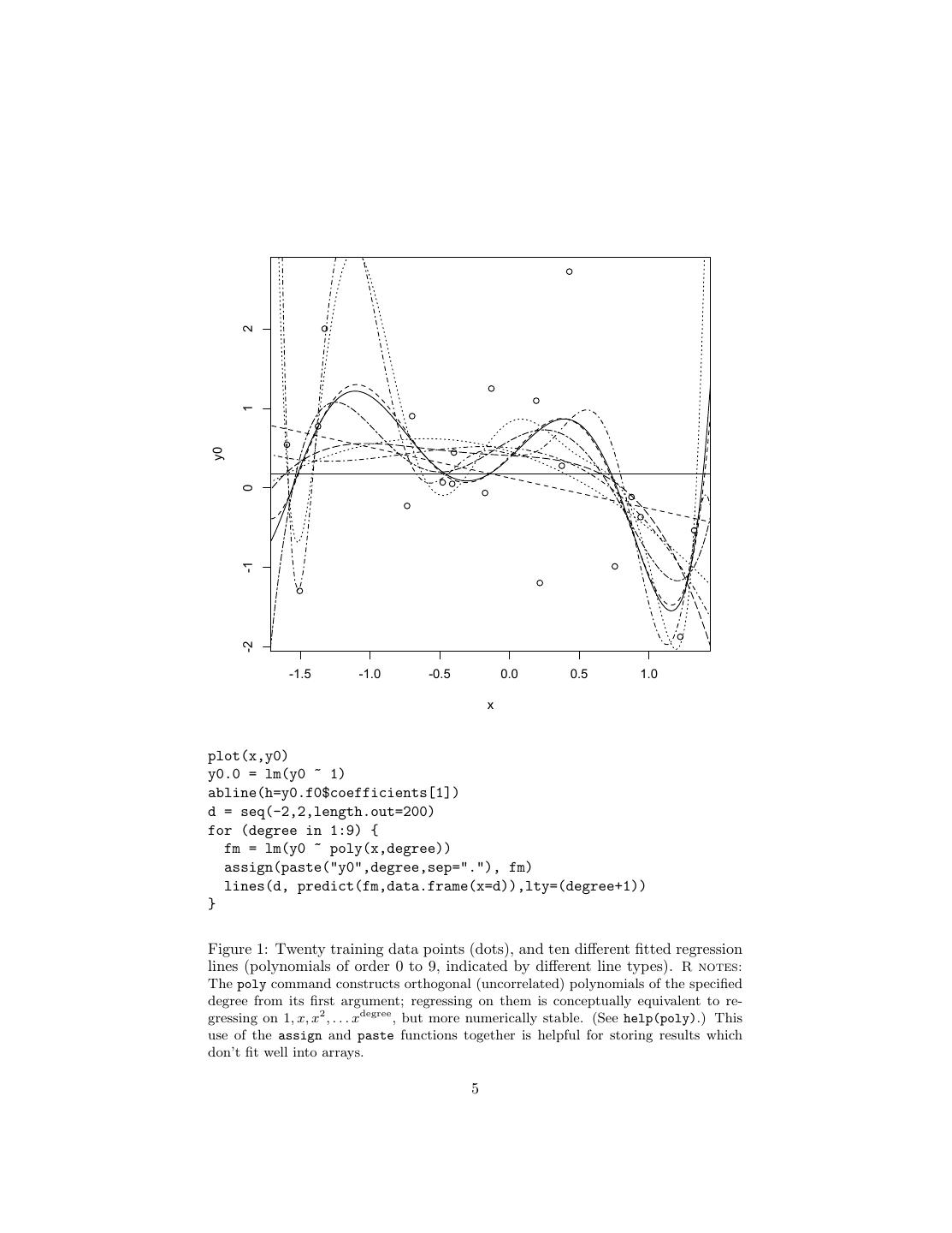
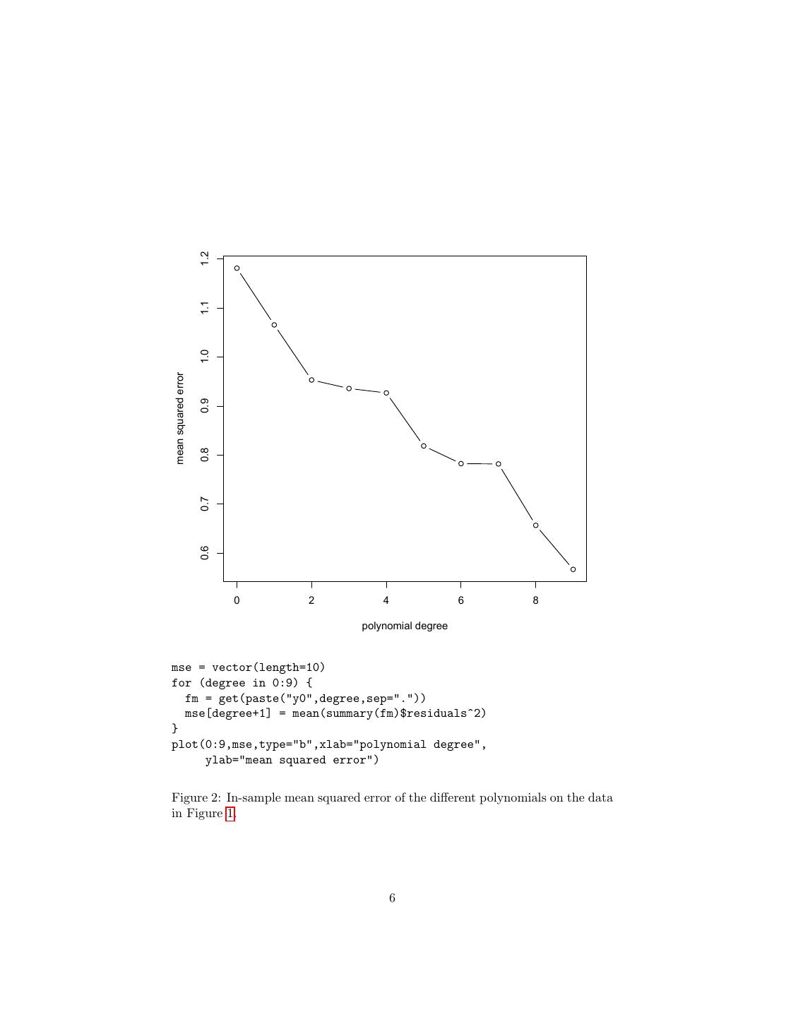
4 .probability distribution. (I write it ηn (θ) as a reminder that different models are going to be affected differently by the same sampling fluctuations.) The problem, then, is that the model which minimizes the in-sample loss could be one with good generalization performance (E [L(X, θ)] is small), or it could be one which got very lucky (ηn (θ) was large and negative): θ = argmin E [L(X, θ)] + ηn (θ) (2) θ∈Θ We hope that ηn (θ) → 0 as n → ∞. This hope rests on the law of large numbers, at least if the error measure L is not too complicated. This is not quite enough for empirical risk minimization to work, i.e., for the parameter value which minimizes the in-sample risk to converge on the one which minimizes the risk. The complication is that the rate at which ηn (θ) goes to zero can depend on θ. The faster the rate at which these fluctuations die away, the easier it is to estimate a model’s generalization error. When the rates change with θ, it becomes unclear whether a model which did well in-sample is really good, or just from a part of the parameter space where performance is hard to discern. In other words we need ηn (θ) → 0, even though θ tends to pick out the θ with the biggest negative fluctuation η. The main tools of statistical learning theory are therefore uniform laws of large numbers, which control the size of the fluctuations ηn (θ) for all θ simultaneously. Learning theory is a beautiful, deep, and practically important subject, but also subtle and involved one.6 Rather than try to explain Vapnik-Chervonenkis dimension and empirical process theory at this level, I will stick with some more- or-less heuristic methods, which are generally good enough for many purposes. 2 Some Examples: Over-Fitting and Under-Fitting To see how these distinctions between in-sample and generalization performance can matter, consider choosing among different classes of models — also called model selection. We are fortunate enough to have in our possession twenty labeled data points, with covariates and a response, and all we have to do is guess the response variable. We recognize this as a supervised learning problem, specifically regression, so we try different regression models. In fact, we try ten different polynomial regressions, running from a constant prediction through a linear model up to polynomials of order nine. Figure 1 shows the results. Looking at the figure suggests that the higher-order polynomials give better fits. In fact, this has to be true, since we’re (i) looking for the best-fitting polynomial of a given order, and (ii) every lower-order polynomial is a special case of the higher-order ones. We can confirm this by looking at the mean squared error (= residual sum of squares/n), as in Figure 2. 6 Some comparatively easy starting points are Kearns and Vazirani (1994) or Cristianini and Shawe-Taylor (2000). At a more advanced level, look at the review paper by Bousquet et al. (2004), or the textbook by Vidyasagar (2003), or read the book by Vapnik (2000) (one of the founders), or take the class 36-712. 4 

5 . 2 1 y0 0 -1 -2 -1.5 -1.0 -0.5 0.0 0.5 1.0 x plot(x,y0) y0.0 = lm(y0 ~ 1) abline(h=y0.f0$coefficients[1]) d = seq(-2,2,length.out=200) for (degree in 1:9) { fm = lm(y0 ~ poly(x,degree)) assign(paste("y0",degree,sep="."), fm) lines(d, predict(fm,data.frame(x=d)),lty=(degree+1)) } Figure 1: Twenty training data points (dots), and ten different fitted regression lines (polynomials of order 0 to 9, indicated by different line types). R notes: The poly command constructs orthogonal (uncorrelated) polynomials of the specified degree from its first argument; regressing on them is conceptually equivalent to re- gressing on 1, x, x2 , . . . xdegree , but more numerically stable. (See help(poly).) This use of the assign and paste functions together is helpful for storing results which don’t fit well into arrays. 5 

6 . 1.2 1.1 1.0 mean squared error 0.9 0.8 0.7 0.6 0 2 4 6 8 polynomial degree mse = vector(length=10) for (degree in 0:9) { fm = get(paste("y0",degree,sep=".")) mse[degree+1] = mean(summary(fm)$residuals^2) } plot(0:9,mse,type="b",xlab="polynomial degree", ylab="mean squared error") Figure 2: In-sample mean squared error of the different polynomials on the data in Figure 1. 6 

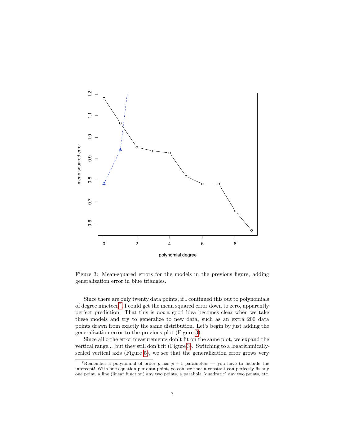
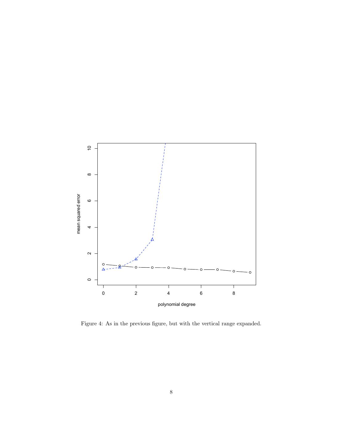
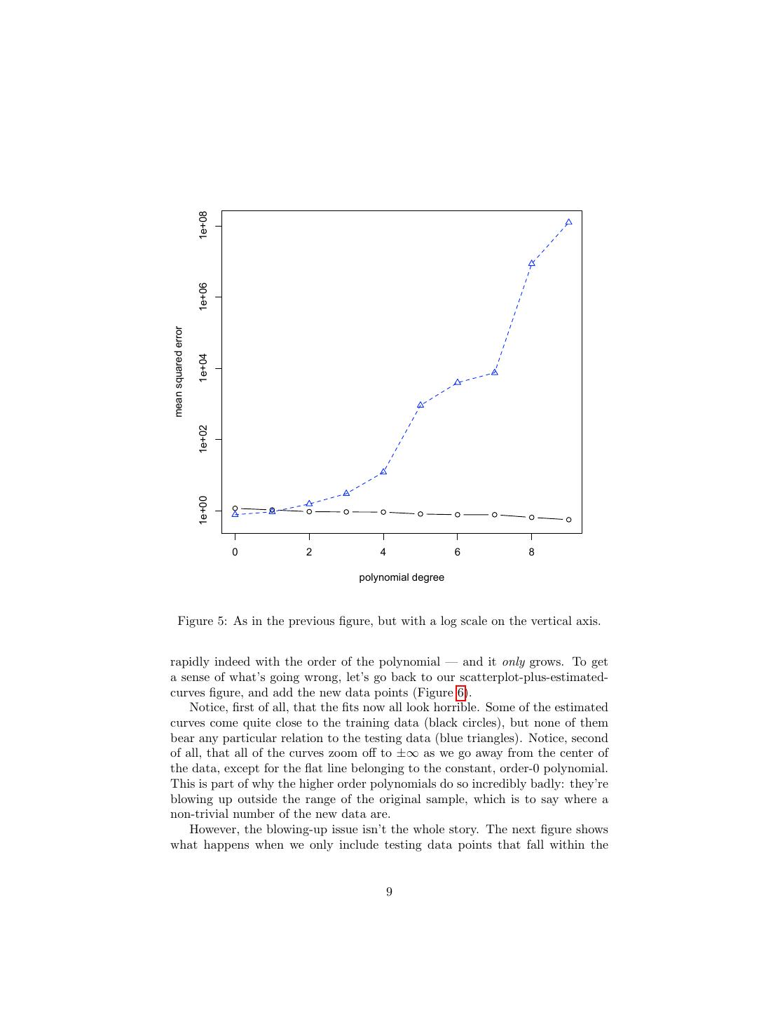
7 . 1.2 1.1 1.0 mean squared error 0.9 0.8 0.7 0.6 0 2 4 6 8 polynomial degree Figure 3: Mean-squared errors for the models in the previous figure, adding generalization error in blue triangles. Since there are only twenty data points, if I continued this out to polynomials of degree nineteen7 , I could get the mean squared error down to zero, apparently perfect prediction. That this is not a good idea becomes clear when we take these models and try to generalize to new data, such as an extra 200 data points drawn from exactly the same distribution. Let’s begin by just adding the generalization error to the previous plot (Figure 3). Since all o the error measurements don’t fit on the same plot, we expand the vertical range... but they still don’t fit (Figure 3). Switching to a logarithmically- scaled vertical axis (Figure 5), we see that the generalization error grows very 7 Remember a polynomial of order p has p + 1 parameters — you have to include the intercept! With one equation per data point, yo can see that a constant can perfectly fit any one point, a line (linear function) any two points, a parabola (quadratic) any two points, etc. 7 

8 . 10 8 mean squared error 6 4 2 0 0 2 4 6 8 polynomial degree Figure 4: As in the previous figure, but with the vertical range expanded. 8 

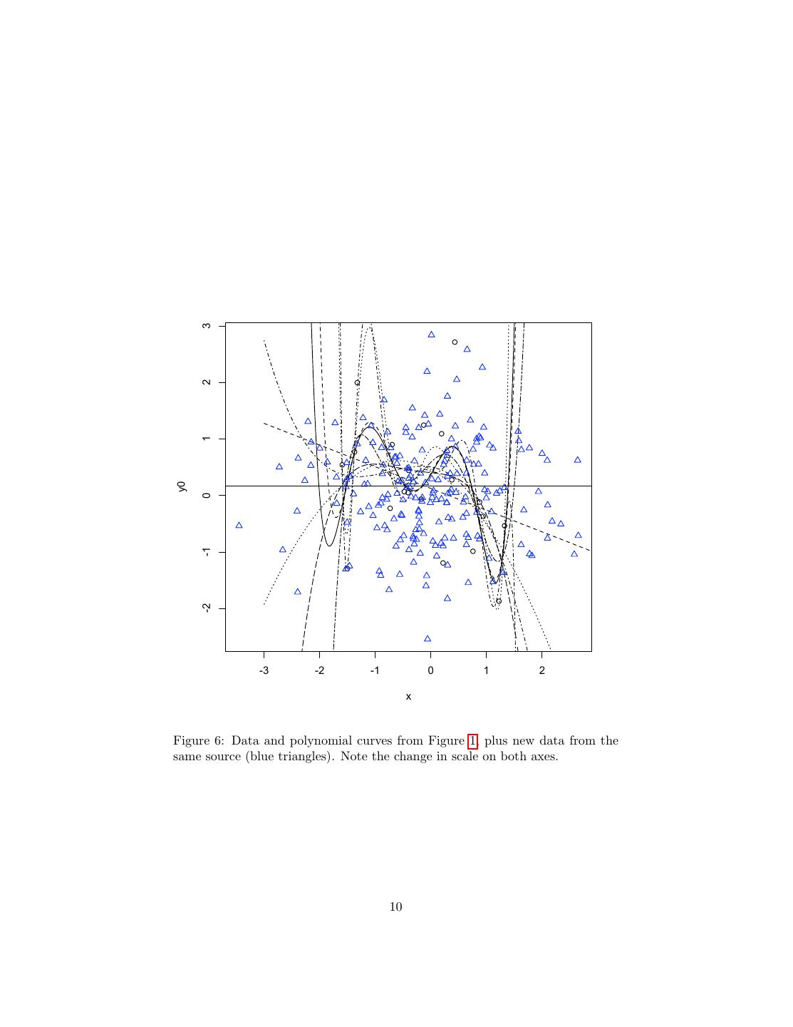
9 . 1e+08 1e+06 mean squared error 1e+04 1e+02 1e+00 0 2 4 6 8 polynomial degree Figure 5: As in the previous figure, but with a log scale on the vertical axis. rapidly indeed with the order of the polynomial — and it only grows. To get a sense of what’s going wrong, let’s go back to our scatterplot-plus-estimated- curves figure, and add the new data points (Figure 6). Notice, first of all, that the fits now all look horrible. Some of the estimated curves come quite close to the training data (black circles), but none of them bear any particular relation to the testing data (blue triangles). Notice, second of all, that all of the curves zoom off to ±∞ as we go away from the center of the data, except for the flat line belonging to the constant, order-0 polynomial. This is part of why the higher order polynomials do so incredibly badly: they’re blowing up outside the range of the original sample, which is to say where a non-trivial number of the new data are. However, the blowing-up issue isn’t the whole story. The next figure shows what happens when we only include testing data points that fall within the 9 

10 . 3 2 1 y0 0 -1 -2 -3 -2 -1 0 1 2 x Figure 6: Data and polynomial curves from Figure 1, plus new data from the same source (blue triangles). Note the change in scale on both axes. 10 

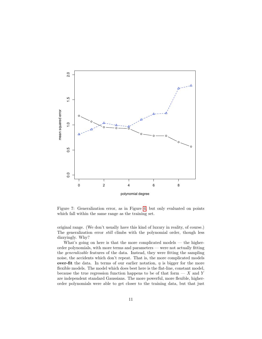
11 . 2.0 1.5 mean squared error 1.0 0.5 0.0 0 2 4 6 8 polynomial degree Figure 7: Generalization error, as in Figure 4, but only evaluated on points which fall within the same range as the training set. original range. (We don’t usually have this kind of luxury in reality, of course.) The generalization error still climbs with the polynomial order, though less dizzyingly. Why? What’s going on here is that the more complicated models — the higher- order polynomials, with more terms and parameters — were not actually fitting the generalizable features of the data. Instead, they were fitting the sampling noise, the accidents which don’t repeat. That is, the more complicated models over-fit the data. In terms of our earlier notation, η is bigger for the more flexible models. The model which does best here is the flat-line, constant model, because the true regression function happens to be of that form — X and Y are independent standard Gaussians. The more powerful, more flexible, higher- order polynomials were able to get closer to the training data, but that just 11 

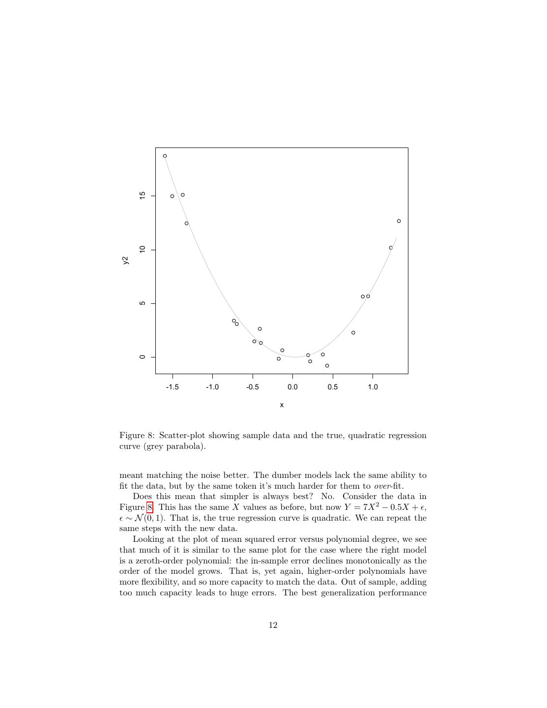
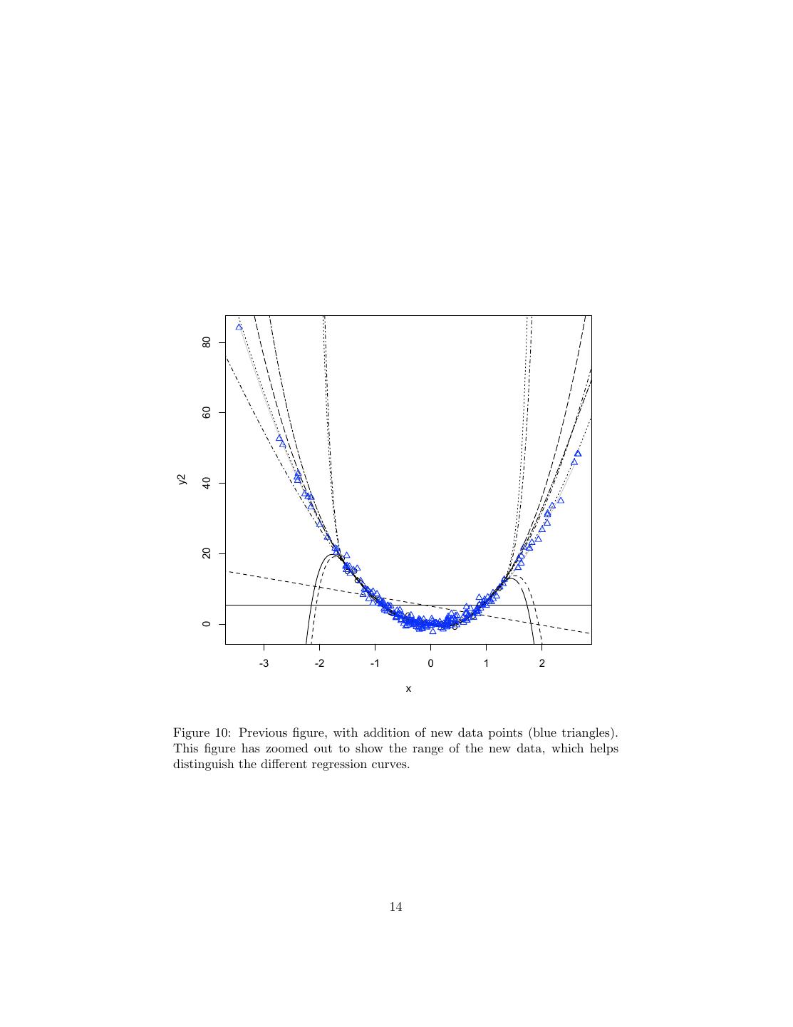
12 . 15 10 y2 5 0 -1.5 -1.0 -0.5 0.0 0.5 1.0 x Figure 8: Scatter-plot showing sample data and the true, quadratic regression curve (grey parabola). meant matching the noise better. The dumber models lack the same ability to fit the data, but by the same token it’s much harder for them to over-fit. Does this mean that simpler is always best? No. Consider the data in Figure 8. This has the same X values as before, but now Y = 7X 2 − 0.5X + , ∼ N (0, 1). That is, the true regression curve is quadratic. We can repeat the same steps with the new data. Looking at the plot of mean squared error versus polynomial degree, we see that much of it is similar to the same plot for the case where the right model is a zeroth-order polynomial: the in-sample error declines monotonically as the order of the model grows. That is, yet again, higher-order polynomials have more flexibility, and so more capacity to match the data. Out of sample, adding too much capacity leads to huge errors. The best generalization performance 12 

13 . 15 10 y2 5 0 -1.5 -1.0 -0.5 0.0 0.5 1.0 x Figure 9: Polynomial fits to the data in the previous figure. 13 

14 . 80 60 y2 40 20 0 -3 -2 -1 0 1 2 x Figure 10: Previous figure, with addition of new data points (blue triangles). This figure has zoomed out to show the range of the new data, which helps distinguish the different regression curves. 14 

15 . 200 1e+06 150 mean squared error mean squared error 1e+04 100 1e+02 50 1e+00 0 0 2 4 6 8 0 2 4 6 8 polynomial degree polynomial degree Figure 11: In-sample and generalization error for the quadratic case. The left- hand plot shows the mean squared error (black for in-sample, blue for general- ization) on a linear scale; the right-hand plot uses a logarithmic scale. comes from using the right model class (here, second-order polynomials). The difference, now, is that it’s possible to have too little capacity, as with zeroth- and first- order models. These also do badly on future data, because they are under-fit. This is the more usual case; when we can plot the generalization error versus model capacity, it usually has a minimum. In these two cases, we get our best generalization performance by using the correct model class. This is possible because our models are well-specified. What if the true regression function does not belong to any class of model available to us? Then there is still generally a capacity/error minimum, but the location of the minimum, i.e., which model class generalizes best, can depend on the sample size. To understand why, remember that we can always decompose the mean- squared error into bias (squared) plus variance. (Similar decompositions hold for other error measures.) If none of our model classes contain the truth, they are all more or less biased; the size of the bias does not, however, depend on n — it’s basically the mis-match between the best model in that class and the truth. The variance term does depend on n — it’s related to ηn (θ) (call this ηn for short). Since high-capacity models start with large values of ηn when n is small, their total generalization error can be larger than that of low-capacity models. As n grows, however, their variance penalty ηn declines, and their superior flexibility (smaller bias) takes over. (If this isn’t clear now, wait for the homework!) There is nothing special about polynomials here. All of the same lessons ap- ply to any other flexible family of models, such as k-nearest neighbors (where we need to choose k), or kernel regression (where we need to choose the bandwidth), or local linear regression (where we need to choose the smoothing range), or fac- 15 

16 .tor analysis (where we need to choose the number of factors), or other methods we’ll see later. 3 Model Selection and Capacity Control The biggest single problem with making data mining work is bad data. The second biggest problem is controlling model capacity, making sure it’s neither so small that we’re missing useful and exploitable patterns, nor so large that we are confusing pattern and noise. How can we do this? 3.1 Big Data The simplest approach to dealing with over-fitting is to hope that it will go away. As we get more and more data, the law of large numbers (and other limit theorems) tell us that it should become more and more representative of the true data-generating distribution, assuming there is one. Thus, η, the difference between the empirical risk and the generalization risk, should grow smaller and smaller. If you are dealing with a lot of data, you can hope that η is very small, and that minimizing the in-sample loss will give you a model which generalizes almost as well as possible. Unfortunately, if your model is very flexible, “lots of data” can be exponentially large. A slightly more subtle point is what happens in cases like the polynomials, where the larger-capacity models always have better fits. Then empirical risk minimization will always select the largest-capacity model class you let it. If that maximum capacity is fixed, this can be OK: suppose the real regression function is quadratic, but we allow polynomials of up to order twenty. Empirical risk minimization will always pick the model of order 20, but as the data grows more and more of the terms in that model (20 − 3 = 17 of them, to be precise) will be shrinking to zero, and we’ll be getting a closer and closer approximation to the correct cubic. If we knew it was a cubic we could do better by setting those terms exactly to zero — they’re adding variance without reducing bias — but, with enough data, the penalty isn’t very big. This same idea can apply even when it seems like we’re not doing model selection, as when we do a big linear regression of a response on a whole mess of variables. With enough data, the coefficients which should be zero will all become small, and have little influence on our predictions, so long as new data has the same distribution as the old. This approach, however, will generally fail if we allow the classes of models to grow too fast as we consider more data, or if we have an infinite collection of model classes to start with. We can always fit n data points exactly with th an (n − 1) order polynomial, so without a limit on the order we always select a curve which goes exactly through the training data and (usually) generalizes horribly. 16 

17 .3.2 Penalization If the problem is over-flexible models, maybe we should penalize flexibility. That is, instead of minimizing L(x, θ), minimize L(x, θ) + λg(θ), where g(θ) is some kind of indication of the complexity or flexibility of θ, say the number of parameters, and λ is our trade-off factor. Standard linear regression packages implement a simple scheme like this in the form of “adjusted R2 .”8 Two more refined ideas for regression are called ridge regression9 , where the penalized error measure is n p 1 2 (yi − xi θ)) + λ θj2 (3) n i=1 j=1 and the lasso, n p 1 2 (yi − xi θ)) + λ |θj | (4) n i=1 j=1 In both cases, the penalty marks down models which give lots of weight to many predictors, compared to those with smaller coefficients but similar errors. The lasso, in particular, tends to shrink regression coefficients to zero when it can. The trade-off here is controlled by λ, which becomes another adjustable control setting, and so it needs to be picked by some other method; the usual approach is cross-validation. Curvature and Splines Another idea is to penalize the curvature of the model: n 1 2 (yi − r(xi , θ)) + λ |∇2 r(z, θ)|dz (5) n i=1 The idea here is that curvature (big second derivatives) is needed to fit very complicated or wiggly functions, but also need to fit noise. By penalizing cur- vature, we allow the regression curve to bend and flex towards the data only if it really improves the fit. (As λ → ∞, we go back towards a linear regression.) It can be shown that the optimal solution is always a piecewise cubic polyno- mial, called a spline10 , which is continuous and has continuous first and second 8 The idea there is that adding an extra predictor variable can never increase the residual sum of squares. (We can always get our old solution back by setting the coefficient equal to zero.) So R2 , in sample, must be a non-decreasing function of the number of independent variables. Assume that the real regression coefficient of the variable we’re adding is zero, and a lot of extra assumptions like independent Gaussian noise, we can calculate the expected increase in R2 when we go from p to p + 1 independent variables, and the true regression coefficient on the (p + 1)th variable is zero. This expected decrease in the RSS is what adjusted R2 is adjusted by. 9 Which we saw when we looked at local linear embedding! 10 Originally, a “spline” was a strip of wood or a board used by draftsmen, carpenters, etc., to draw smooth curves: you pinned it in place at specific points you wanted the curve to go through, and then let it flex. The stiffer the board, the less it would bend — in the mathematical problem, the bigger λ would be. Craftsmen still use them; last year when the 17 

18 .derivatives between the pieces. Such smoothing splines are extremely useful tools, not just for regression but also for classification and density estimation. (The R command smooth.spline will fit a basic smoothing spline to data, but this just scratches the surface.) Splines, generally speaking, provide an alterna- tive to anything one might want to do with kernels, but to handle the properly demands more math than we can presume for this course.11 3.3 From Penalties to Constraints; the Method of Sieves Suppose that instead of penalizing flexibility, we constrained it. Take the lasso; p suppose we constrained g(θ) = j=1 |θj | to be no more than some value c, giving a constraint inequality g(θ) − c ≤ 0. Now we ask for the θ which minimizes the error subject to the constraint: θ = argmin L(x, θ) (6) θ:g(θ)≤c If this was a constraint equation, we’d know how to do the constrained optimiza- tion — we’d just use a Lagrange multiplier. To handle an inequality, we actually do the same thing. Either the function can be minimized without hitting the constraint, in which case the Lagrange multiplier will be zero, or the constrained minimum is on the boundary of the region compatible with the constraint, in which case the Lagrange multiplier is non-zero and we’re doing the g(θ) − c = 0 case. Let’s assume the constraint is binding. The Lagrangian is L(x, θ) + λ(g(θ) − c) = L(x, θ) + λg(θ) − cλ (7) Notice that the last term does not involve θ. This means that, for any given λ, argmin L(x, θ) + λg(θ) = argmin L(x, θ) + λg(θ) − cλ (8) θ θ and we can forget about the cλ term when optimizing over θ. But then we’re back to our penalized optimization problem! In the constrained problem, each value of the constraint c implies a particular value of the multiplier λ, and conversely. How would be pick c? We could just treat it as a fixed value, but let’s recall why we’re doing this. Very flexible models tend to over-fit; as we saw earlier, if we let the collection of models we consider grow too fast with n, then we always overfit and never generalize properly. But if we never let the collection of models increase, we will always be left with some systematic bias, which we could reduce by using more flexible models. (Unless, by some miracle, the truth gas company tore up our driveway and then replaced it, the workmen got rounded edges in the concrete by using big plywood boards as their splines. (Of course our flower-beds had sharp corners and we had to break up the extra concrete with chisels and sledgehammers.) 11 There is a good basic discussion of them in Berk (2008, §2.2 and 2.4). The best single reference is Wahba (1990), but she assumes you know what a Hilbert space is. 18 

19 .is included among our models.) This suggests that the value of the constraint c should actually be allowed to grow with n, that it’s really c(n), with c(n) → ∞ as n → ∞. The story here is that initially we use very highly constrained models, which may miss a lot of features of the data but at least won’t over-fit. Then, as we get more data and it becomes easier to tell signal from noise, we relax the constraint, and pick out finer and finer details of the data. This approach is called the method of sieves, with the sequence of sets of models {θ : g(θ) ≤ c(n)} being the sieve.12 The crucial questions become “what should we constrain?” (what should g(θ)?), and “how quickly can we relax the constraint?” (what should c(n) be?). Designing a good sieve involves answering both these questions, which in turn usually involves understanding the sampling fluctuations ηn (θ) — the trick is to let c(n) grow just slowly enough that the sampling fluctuations still converges to zero. Any slower (say, c(n) = c0 for all n), and we’re suffering from unnecessary bias; any faster, and we’re sucked into overfitting. (We saw that if g(θ) is the order of a polynomial, c(n) = n − 1 is too fast.) While we could explore this, or just present some sieves people have already worked out, I’m going to instead concentrate on other methods where the underlying principles are easier to grasp, but you should in particular be aware of the correspondence between penalties and constraints.13 3.4 Capacity Control Penalization can work very well, but the trick is in choosing the penalty term; the number of parameters is often used but not always appropriate, though it is in the polynomial example. The real issue is what I have already referred to a few times as capacity. Roughly speaking, the idea is that a class of models has high capacity if changing the data a little bit gives rise to a very different model, i.e., one which makes very different predictions. A more exact view is to look at how many distinct models we can get by changing the data, where “distinct” involves setting some threshold on how different the models’ predictions must be. Low-capacity model classes are insensitive to the data, and the number of distinct models grows only slowly with the number of data points. High- capacity model classes are very sensitive to the data.14 The trade-off, again, is between have a (potentially) high bias, and having a high variance — between under-fitting and over-fitting. Capacity, in this sense, is often related to the number of parameters, but not always. There are examples (not crazy ones, even) of model classes with one adjustable parameter whose capacity is, in fact, infinite, making generalization 12 The metaphor behind the name is to imagine sifting something through sieves with finer and finer meshes, catching smaller and smaller things. 13 The method of sieves was supposedly introduced by Grenander (1981), but my impression is that almost nobody has read it (I haven’t); instead it was spread by Geman and Hwang (1982). van de Geer (2000) illustrates the interplay between the method of sieves and advanced convergence theory. 14 To be really precise, we need to consider not just the scaling with the number of data points but also the scaling with the cut-off for being distinct models, except in the case of classification where the outputs are discrete. See Vapnik (2000) for details. 19 

20 .very difficult indeed.15 In the case of things like kernel regression or nearest neighbors, choosing a large neighborhood (high k or high bandwidth) reduces the capacity, by making the model less sensitive to the data. All of this suggests that a reasonable kind of penalty to apply would be an estimate of how big ηn (θ) can get. All else being equal, this will be large for high-capacity model classes, and it will shrink as n grows. Statistical learning theory provides tools for estimating those penalties, and the resulting strategy is called structural risk minimization. However, computing capacity-based penalties is hard, because one needs to know the capacities of different model classes, which are generally quite difficult to compute. (Trust me, or read the references, or take 36-712.) 3.5 Cross-Validation Since we often aren’t in a position to use real capacity-based penalties, what shall we do instead? A short-cut trick, which is often reliable and in some ways is the industry standard, is to simulate the process of fitting to different data sets and seeing how different the predictions can be. Divide your data at random into two parts. Call the first part the train- ing set, and use it to fit your models. Then evaluate their performance on the other part, the testing set. Because you divided the data up randomly, the performance on the test data should be an unbiased estimate of the gen- eralization performance. (But, unbiased doesn’t necessarily mean “close”.) In fact, you can do this multiple times, say selecting 90% of the data at random to be the training set, testing on the remaining 10%, and then repeating this ten times, with different choices of training and test sets, and picking the model which comes out best when averaged over these ten trials; this is called ten-fold cross-validation. (There is nothing magic about ten, it’s just large enough to get a bit of averaging but small enough to usually run in decent time.) The reason cross-validation works is that it uses the existing data to simulate the process of generalizing to new data. If the full sample is large, then even the smaller portion of it in the training data is, with high probability, fairly representative of the data-generating process. Randomly dividing the data into training and test sets makes it very unlikely that the division is rigged to favor any one model class, over and above what it would do on real new data. Of course the original data set is never perfectly representative of the full data, and a smaller testing set is even less representative, so this isn’t ideal, but the approximation is often quite good. (Of course, all of this assumes that the original data is in fact a representative sample of the data we will be applying our models to in the future — that our data-generating process isn’t biased, that there isn’t too much dependence between data points, etc.) 15 The canonical example is to take classifiers which output 1 if sin ax is positive and 0 otherwise. That is, the classes correspond to two halves of a periodic cycle. By adjusting a, one can always match the classes on any collection of binary-labeled data. 20 

21 . Cross-validation is probably the most widely-used method for model selec- tion, and for picking control settings, in all applications of data-mining and machine learning. There are circumstances where it can fail — especially if you give it too many models to pick among — but it’s the first thought of practi- tioners, and it should be your first thought, too. The homework will make you very familiar with it. 3.6 Why Chose? Alternately, we can refuse to pick a model at all, and simply average all the ones we feel like fitting. We’ll say more about this later. 4 Warnings Two caveats are in order. 1. All the model selection methods we have discussed aim at getting models which predict well. This is not necessarily the same as getting the true theory of the world. Presumably the true theory will also predict well, but the converse does not necessarily follow. 2. All of these model selection methods aim at getting models which will generalize well to new data, if it follows the same distribution as old data. Generalizing well even when distributions change is a much harder and much less well-understood problem (Qui˜ nonero-Candela et al., 2009). This relates to the first point, of course. 5 Exercises To think through, not to hand in. 1. Suppose that one of our model classes contains the true and correct model, but we also consider more complicated and flexible model classes. Does the bias-variance trade-off mean that we will over-shoot the true model, and always go for something more flexible, when we have enough data? (This would mean there was such a thing as too much data to be reliable.) 2. The ordinary least squares estimate for the coefficients of linear regres- −1 sion is (xT x) xT y. Find an analogous closed-form expression for ridge regression? Hints: Remember that the answer will have to involve λ, and possibly some other matrices. Also, look at how we used Tikhonov regularization in the handout on local linear embedding. 3. Can you find a closed-form expression for the lasso? 21 

22 . 4. A simple form of cross-validation is called data splitting: make one random division of the data into training and test sets of equal size. Write down a formula for the loss on the testing set in terms of the risk and a sampling fluctuation. How does this compare to the in-sample losses? References Berk, Richard A. (2008). Statistical Learning from a Regression Perspective. Springer Series in Statistics. New York: Springer-Verlag. Bousquet, Olivier, St´ephane Boucheron and G´abor Lugosi (2004). “Introduction to Statistical Learning Theory.” In Advanced Lectures in Machine Learning (Olivier Bousquet and Ulrike von Luxburg and Gunnar R¨atsch, eds.), pp. 169– 207. Berlin: Springer-Verlag. URL http://www.econ.upf.edu/~lugosi/ mlss_slt.pdf. Cristianini, Nello and John Shawe-Taylor (2000). An Introduction to Support Vector Machines: And Other Kernel-Based Learning Methods. Cambridge, England: Cambridge University Press. Geman, Stuart and Chii-Ruey Hwang (1982). “Nonparametric Maximum Like- lihood Estimation by the Method of Sieves.” The Annals of Statistics, 10: 401–414. URL http://projecteuclid.org/euclid.aos/1176345782. Grenander, Ulf (1981). Abstract Inference. New York: Wiley. Kearns, Michael J. and Umesh V. Vazirani (1994). An Introduction to Compu- tational Learning Theory. Cambridge, Massachusetts: MIT Press. Qui˜ nonero-Candela, Joaquin, Masashi Sugiyama, Anton Schwaighofer and Neil D. Lawrence (eds.) (2009). Dataset Shift in Machine Learning. Cam- bridge, Massachusetts: MIT Press. van de Geer, Sara (2000). Empirical Processes in M-Estimation. Cambridge, England: Cambridge University Press. Vapnik, Vladimir N. (2000). The Nature of Statistical Learning Theory. Berlin: Springer-Verlag, 2nd edn. Vidyasagar, M. (2003). Learning and Generalization: With Applications to Neural Networks. Berlin: Springer-Verlag, 2nd edn. Wahba, Grace (1990). Spline Models for Observational Data. Philadelphia: Society for Industrial and Applied Mathematics. 22