Improving the Query Performance of High-Dimensional Index Struct

1 . Improving the Query Performance of High-Dimensional Index Structures by Bulk Load Operations Stefan Berchtold 1, Christian BShm 2, and Hans-Peter Kriegel 2 1 AT&T Labs Research, 180 Park Avenue, Florham Park, NJ 07932 2 University of Munich, Oettingenstr. 67, D-80638 Miinchen Abstract. In this paper, we propose a new bulk-loading technique for high-di- mensional indexes which represent an important component of multimedia data- base systems. Since it is very inefficient to construct an index for a large amount of data by dynamic insertion of single objects, there is an increasing interest in bulk-loading techniques. In contrast to previous approaches, our technique ex- ploits a priori knowledge of the complete data set to improve both construction time and query performance. Our algorithm operates in a mannar similar to the Quicksort algorithm and has an average runtime complexity of O(n log n). We ad- ditionally improve the query performance by optimizing the shape of the bound- ing boxes, by completely avoiding overlap, and by clustering the pages on disk. As we analytically show, the split strategy typically used in dynamic index struc- tures, splitting the data space at the 50%-quantile, results in a bad query perfor- mance in high-dimensional spaces. Therefore, we use a sophisticated unbalanced split strategy, which leads to a much better space partitioning. An exhaustive ex- perimental evaluation shows that our technique clearly outperforms both classic index construction and competitive bulk loading techniques. In comparison with dynamic index construction we achieve a speed-up factor of up to 588 for the con- struction time. The constructed index causes up to 16.88 times fewer page access- es and is up to 198 times faster (real time) in query processing. 1. Introduction Multimedia database systems gain more and more importance in both database research and industry. In contrast to standard database systems, multimedia applications require similarity search as a basic functionality. A widely applied technique for searching a mul- timedia database for similar objects is the so-called feature transformation where important properties of the database object are transformed into a high-dimensional point, the so-called feature vector [10, 15, 18]. Usually, multidimensional index structures are used to manage the set of feature vectors. Most of the research regarding multidimension- al index structures [1, 5, 4, 19, 14] focuses on a good search performance. Therefore, the performance of the proposed index structures for insert operations is sufficient only when inserting a relatively small amount of data, e.g. a single data item [4, 14]. A typical data- base application, however, starts with an empty database which will continuously grow due to multiple insert operations. It is not appropriate to use an index structure in the be- ginning of this process because having only a relatively small amount of high- dimensional feature vectors, a sequential scan of the data will be much faster than an in- dex based search [7, 2]. However, if the size of the database reaches a certain threshold, the use of an index structure is required. In another scenario, we might want to replace a legacy system managing a large amount of data by a multimedia database system. In both cases, we face the problem to build an index file from a large amount of data i.e. to bulk- load the index. 

2 . 217 On the other hand, we may draw some advantage from the fact that we do not only know a single data item - as in case of a normal insertion operation - but a large amount of data items. It is common knowledge that we can achieve a higher fanout and storage utili- zation using bulk load operations resulting in a slightly better search performance. But, do we exhaust all the potential of this information by increasing the storage utilization? As we show in this paper, we do not. In this paper, we propose a new bulk-loading technique L for R-tree-like index struc- tures. In contrast to other bulk-loading techniques, our algorithm exploits a priori knowledge of the complete data set to achieve a better data space partitioning. An arbi- trary storage utilization can be chosen, including a near-100% 2 utilization. Furthermore, if we choose a storage utilization lower than 100%, we use the gained freedom for an ac- celeration of the construction. During the bulk-load operation, the complete data is held on secondary storage. Therefore, only a small cache in main memory is required and cost intensive disk operations such as random seeks are minimized. The basic idea of our tech- nique is to split the data space recursively in a top-down fashion using hyperplanes as separators between the partitions. The hyperplanes are defined by a split dimension (the normal vector of the hyperplane) and a split value (defining the actual location of the hy- perplane). Space partitioning is done by an algorithm that is similar to the well-known Quicksort algorithm although operating on secondary storage. Our technique is invariant against a specific split strategy i.e., gives us the freedom to partition the space according to arbitrary split dimensions and split values. W e use this freedom to create a optimized space partitioning that is unbalanced and therefore cannot be achieved by a dynamic in- dex structure. Note that, although partitioning is unbalanced, our algorithm guarantees that the resulting index structure is balanced. The paper is concluded by a variety of ex- perimental results that demonstrate the advantage of our technique in comparison with dynamic indexing and other bulk loading techniques. W e analytically show in Appendix A that our bulk-load operation can be done in average O(n log n) time. 2. Bulk-loading Multidimensional Index Structures In this section, we will give an overview of the related research: A variety of high-dimen- sional index structures has been proposed in the past. The most well-known index structures are the TV-tree [ 14], the S S-tree [ 19], the S R-tree [ 13] and the X-tree [4]. How- ever, none of these index structures supports an efficient bulk-load operation by itself. On the other hand, some bulk-load techniques have been proposed. For example, the Hilbert R-tree [12] is created by externally sorting all the data vectors according to their Hilbert value and assigning equally sized, subsequential portions of the sorted data to data pages. Finally, the bounding boxes of the data pages are stored in directory pages cluster- ing these directory pages recursively until we reach a single root node. The costs for bulk loading a Hilbert R-tree are obviously in O(n log n) due to external sorting. However, a 1. Frequently, bulk-loading an index is also called bottom-up construction of the index because we first construct the data pages which are at the "bottom" of the index structure and then construct the directory pages. As this term is misleading because we actually partition the data space in a top-down fashion, we omit this term and use bulk-loading or simply index construction instead. 2. "near 100%" means 100% up to round-up effects. 

3 . 218 major drawback of the Hilbert R-tree is that Hilbert ordering degenerates in higher di- mensions leading to a bad query performance. As an alternative, we can divide the data space into partitions that correspond to data pages. This partitioning of the data space can be done in a top-down fashion which means that we hierarchically divide the d-dimensional space using (d-1)-dimensional hyper- planes as borderlines between the partitions. In addition, however, we have to assure that a directory can be built on top of this space partitioning. In [11], Jain and White intro- duced the VAM-Split R-tree and the VAM-Split KD-tree. VAM-Split trees are rather similar to KD-trees [16], however in contrast to KD-trees, split dimensions are not chosen in a round robin fashion but depending on the maximum variance. VAM Split trees are built in main memory and then stored to secondary storage. Therefore, the size of a VAM- Split tree is limited by the available main memory. In [6], van den Bercken, Seeger and Widmayer proposed buffer trees which potential- ly work on all multidimensional index structures. The buffer tree is a derivative of the data structure to be constructed with two major modifications: First, an additional buffer is assigned to every directory page, and second, the capacity of a directory page may dif- fer from the capacity of the target index structure. The buffer of every directory page is partially held in main memory and partially laid out on secondary storage. During the bulk load, each tuple is inserted into the buffer of the root node. If the buffer of the root node overflows, all objects in the buffer are dispatched to the next deeper index level. This process continues until the data level is reached. The general advantage of the buffer tree approach is that algorithms designed for tuning the query performance of the target index structure can be applied without modification. Obviously, the resulting index has the same properties as a dynamically constructed index. None of these algorithms, however, uses the available knowledge of a large amount of data to improve the performance of the resulting index structure. 3. Our New Technique In this section, we present our new bulk-loading technique. The index construction algo- rithm is a recursive algorithm comprising the following subtasks: 9 determining the tree topology (height, fanout of the directory nodes, etc.) 9 the split strategy 9 external bisection of the data set on secondary storage 9 constructing the index directory. Although all these subtasks run in a nested fashion, we will present them separately to maintain clarity. However, we cannot regard the split strategy and the bisection indepen- dently from the tree topology. For example, we can only determine the exact topology of a subtree if we know the exact number of data objects stored in this subtree. This exact number, however, depends on the results of previous splits and bisections. Thus, although we separately describe the parts of the algorithms, we have to keep in mind the special requirements and prerequisites of the other parts. An example will clarify the idea of our algorithm: Let us assume that we have given 10,000 two-dimensional data items and we can take from several properties our index structures that 10,000 items will fill a tree of height 3 having 6 entries in the root node (determination of tree topology). Thus, we first call the recursive partitioning algorithm 

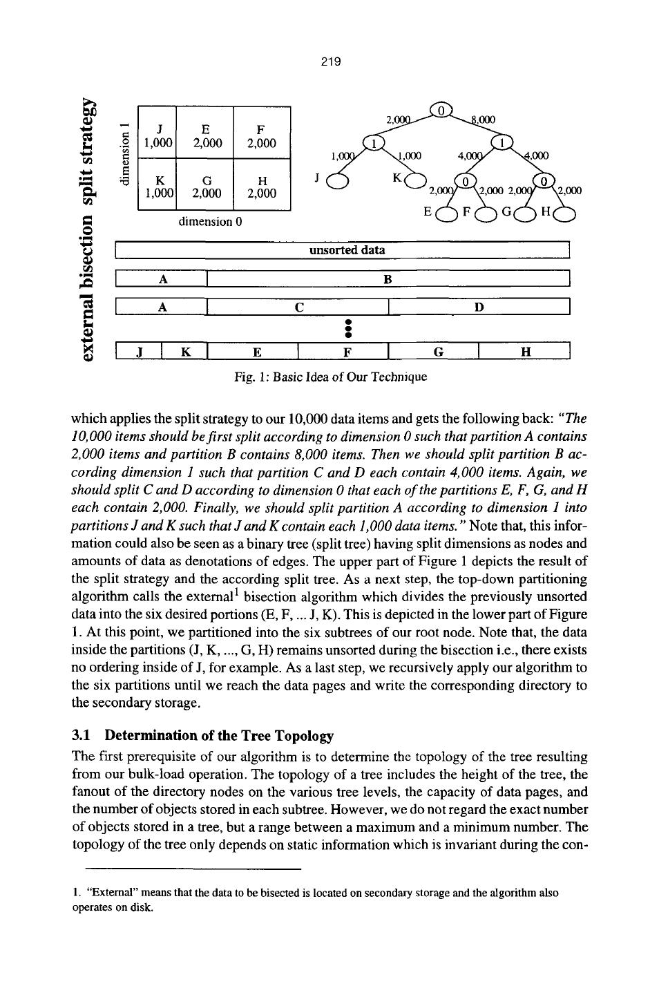
4 . 219 2, ,000 J E F .~ 1,000 2,000 2,000 ~D ~3 K G H rJl 1,000 2,000 2,000 dimension 0 61l unsorted data ,Jl A B A c I D JI K G I " Fig. 1: Basic Idea of Our Technique which applies the split strategy to our 10,000 data items and gets the following back: "The 10, 000 items should be first split according to dimension 0 such that partition A contains 2,000 items and partition B contains 8,000 items. Then we should split partition B ac- cording dimension 1 such that partition C and D each contain 4,000 items. Again, we should split C and D according to dimension 0 that each of the partitions E, F, G, and H each contain 2,000. Finally, we should split partition A according to dimension 1 into partitions J and K such that J and K contain each 1,000 data items." Note that, this infor- mation could also be seen as a binary tree (split tree) having split dimensions as nodes and amounts of data as denotations of edges. The upper part of Figure 1 depicts the result of the split strategy and the according split tree. As a next step, the top-down partitioning algorithm calls the external 1 bisection algorithm which divides the previously unsorted data into the six desired portions (E, F .... J, K). This is depicted in the lower part of Figure 1. At this point, we partitioned into the six subtrees of our root node. Note that, the data inside the partitions (J, K ..... G, H) remains unsorted during the bisection i.e., there exists no ordering inside of J, for example. As a last step, we recursively apply our algorithm to the six partitions until we reach the data pages and write the corresponding directory to the secondary storage. 3.1 Determination of the Tree Topology The first prerequisite of our algorithm is to determine the topology of the tree resulting from our bulk-load operation. The topology of a tree includes the height of the tree, the fanout of the directory nodes on the various tree levels, the capacity of data pages, and the number of objects stored in each subtree. However, we do not regard the exact number of objects stored in a tree, but a range between a maximum and a minimum number. The topology of the tree only depends on static information which is invariant during the con- 1. "External" means that the data to be bisected is located on secondary storage and the algorithm also operates on disk. 

5 . 220 struction such as the number of objects, the dimension of the data space, the page capacity and the storage utilization. Let Cmax,data be the maximum number of data objects in a data page where = I pagesize I, Cmax.data ~_s i z e o ~ j e c t ) _ ] Cmax,dir analogously the maximum fanout of a directory page, and Ceff,data and Ceff,dir the average capacity of a data/directory page with Ceff,data = st~176 Cmax.data" The maximum number of data objects stored in a tree with height h then is: h-I h-1 Cmax,tree(h) = Cmax,data" Cmax,dir Ceff, tree(h) = Ceff, data " Ceff, dir" Therefore, the height of the tree must initially be determined such that Ceff,tree is greater than the actual number of objects n. More formally: h = [logc~ff~r(~)]+l | ' eft,data] Note that we have to evaluate this formula only once in order to determine the level of the root node of the index. As the X-tree and other R-tree related index structures are al- ways height-balanced, we can easily determine the level of subtrees by decrementing the level of the parent node of the subtree. Now, we have to determine the fanout of the root node of a tree T with height h when filled with n data objects. Let us assume that every subtree of height (h-l) is filled according to its average capacity Ceff,tree(h- 1). Thus, the fanout is the quotient of n and the average capacity of the subtrees: fan~ = min(r n ] Cmaxdir) = min([ -- h-2 1" Cmax' l d' ir) /Ceff, tree(h- 1) ' Ceff, data. Ceff,dir Obviously, a 100% storage utilization in every node can be achieved only for certain values of n. Usually, the number of nodes in each level must be rounded-up. Thus, the data nodes and their parents are utilized best according to the desired storage utilization while the worst utilization typically occurs in the top levels of the tree. In general, our al- gorithm creates the highest possible average storage utilization below the chosen one. 3.2 The Split Strategy Once we laid down the f a n o u t f o f a specific directory page P, the split strategy has to be applied to determinef subsets of the current data. As we regard the split strategy as an re- placeable part of our algorithm, we only describe the requirements of a split strategy in this section. A detailed description of our optimized split strategy we be given in section 4. Assuming that the dataset is bisected repeatedly, the split strategy determines the bi- nary split tree for a directory page, which has f leaf nodes and may be arbitrarily unbalanced. Each non-leaf node in the split tree represents a hyperplane (the split plane) splitting the data set into two subsets. The split plane can be described by the split dimen- sion and the numbers of data objects (NDO) on each side of the split plane. Thus, a split strategy has to determine the split dimension and the ratio between the two NDOs. Fur- thermore, we allow the split strategy to produce not only constant ratio but a interval of acceptable ratios. We will use this freedom later, to accelerate the bisection algorithm. 1. The minimum is required due to round-offeffects 

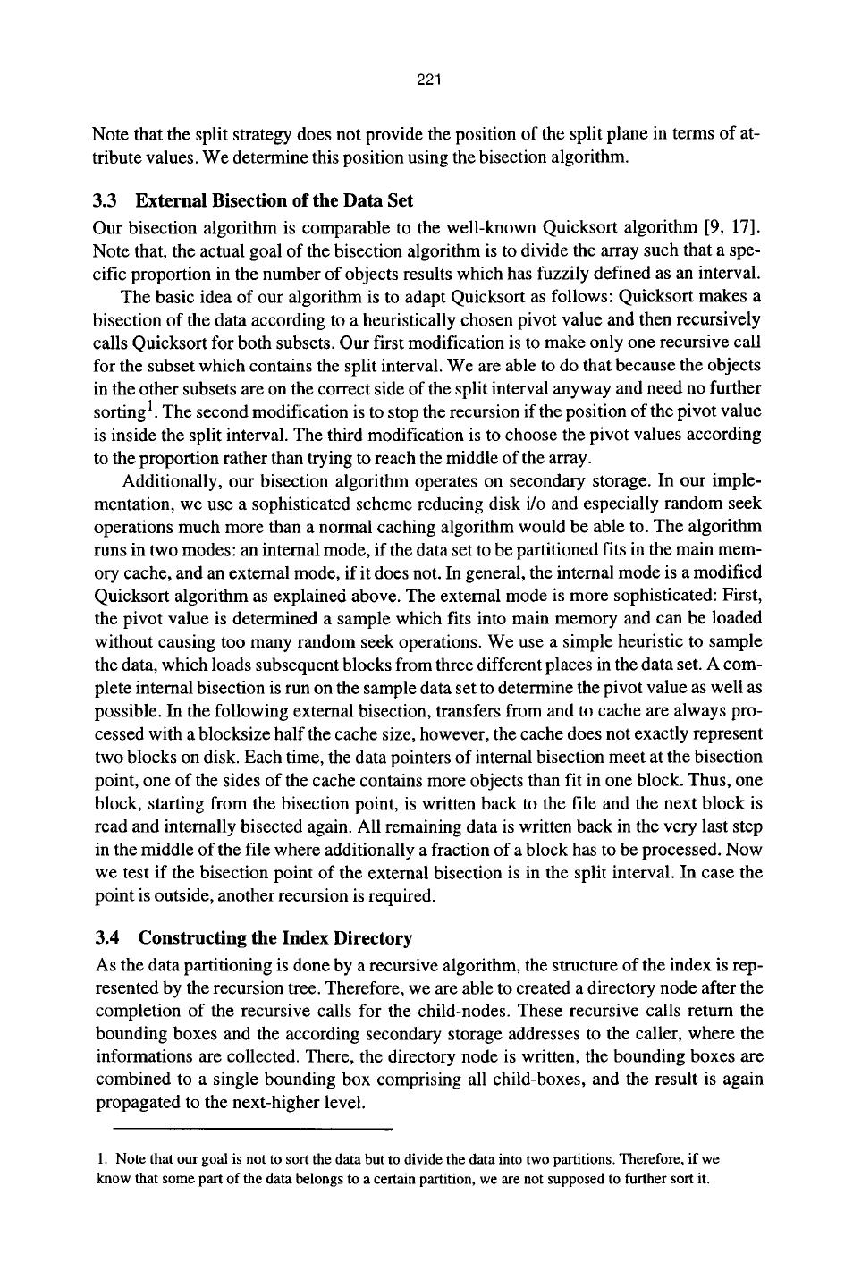
6 . 221 Note that the split strategy does not provide the position of the split plane in terms of at- tribute values. W e determine this position using the bisection algorithm. 3.3 External Bisection of the Data Set Our bisection algorithm is comparable to the well-known Quicksort algorithm [9, 17]. Note that, the actual goal of the bisection algorithm is to divide the array such that a spe- cific proportion in the number of objects results which has fuzzily defined as an interval. The basic idea of our algorithm is to adapt Quicksort as follows: Quicksort makes a bisection of the data according to a heuristically chosen pivot value and then recursively calls Quicksort for both subsets. Our first modification is to make only one recursive call for the subset which contains the split interval. W e are able to do that because the objects in the other subsets are on the correct side of the split interval anyway and need no further sorting 1. The second modification is to stop the recursion if the position of the pivot value is inside the split interval. The third modification is to choose the pivot values according to the proportion rather than trying to reach the middle of the array. Additionally, our bisection algorithm operates on secondary storage. In our imple- mentation, we use a sophisticated scheme reducing disk i/o and especially random seek operations much more than a normal caching algorithm would be able to. The algorithm runs in two modes: an internal mode, if the data set to be partitioned fits in the main mem- ory cache, and an external mode, if it does not. In general, the internal mode is a modified Quicksort algorithm as explained above. The external mode is more sophisticated: First, the pivot value is determined a sample which fits into main memory and can be loaded without causing too many random seek operations. We use a simple heuristic to sample the data, which loads subsequent blocks from three different places in the data set. A com- plete internal bisection is run on the sample data set to determine the pivot value as well as possible. In the following external bisection, transfers from and to cache are always pro- cessed with a blocksize half the cache size, however, the cache does not exactly represent two blocks on disk. Each time, the data pointers of internal bisection meet at the bisection point, one of the sides of the cache contains more objects than fit in one block. Thus, one block, starting from the bisection point, is written back to the file and the next block is read and internally bisected again. All remaining data is written back in the very last step in the middle of the file where additionally a fraction of a block has to be processed. Now we test if the bisection point of the external bisection is in the split interval. In case the point is outside, another recursion is required. 3.4 Constructing the Index Directory As the data partitioning is done by a recursive algorithm, the structure of the index is rep- resented by the recursion tree. Therefore, we are able to created a directory node after the completion of the recursive calls for the child-nodes. These recursive calls return the bounding boxes and the according secondary storage addresses to the caller, where the informations are collected. There, the directory node is written, the bounding boxes are combined to a single bounding box comprising all child-boxes, and the result is again propagated to the next-higher level. 1. Note that our goal is not to sort the data but to divide the data into two partitions. Therefore, if we know that some part of the data belongs to a certain partition, we are not supposed to further sort it. 

7 . 222 Thus, a depth-first post-order sequentialization of the index is written to disk. The se- quentialization starts with a sequence of datapages, followed by the directory-page which is the common parent of these data pages. A sequence of such blocks is followed by a sec- ond-level directory page, and so on. The root page of the directory is the last page in the index file. As geometrically neighboring data pages are also likely to be in the same hier- archical branch, they are well clustered. 4. Improving the Query Performance In dynamic index construction, the most important decision in split processing is the choice of the split axis whereas the split value is rather limited. Heavily unbalanced splits, such as a 10:1 proportion are commonly regarded as undesired because storage utilization guarantees would become impossible, if pages with deliberately low filling degree are generated in an uncontrolled manner. Moreover, for low-dimensional spaces, it is bene- ficial to minimize the perimeter of the bounding boxes i.e., to shape the bounding boxes such that all sides have approximately the same length [5]. But, there are some effects in high-dimensional data spaces leading to performance deterioration when minimizing the perimeter. The first observation in a high-dimensional index is that, at least when applying bal- anced partitioning on a uniformly distributed dataset, the data space cannot be split in each dimension. Assuming for example a 20-dimensional data space which has been split exactly once in each dimension, would require 220 = 1,000,000 data pages or 30,000,000 objects if the effective page capacity is 30 objects. Therefore, the data space is usually split once in a number d' of dimensions. In the remaining (d - d') dimensions it has not been split and the bounding boxes include almost the whole data space in these dimen- sions. As we assume the d-dimensional unit hypercube as data space, the bounding boxes have approximately side length 1/2 in d' dimensions and approximately side length 1 in (d - d') dimensions. The maximum split dimension d' can be determined from the number N of objects stored in the database: d' = log2(~-N ). 1 ~ eff The second observation is that a similar property holds for typical range queries. If we assume that the range query is a hypercube and should have a selectivity s, then the side length q is the d th root of s: q = d~. For a 20-dimensional range query with selectivity 0.01% we get a side length q = 0.63 which is larger than half of the extension of the data space in this direction. It becomes intuitively clear that a query with side length larger than 1/2 must intersect with every bounding box having at least side length 0.5 in each dimension. However, we are also able to model this effect more accurate: The performance of a multi-dimensional range query is usually modeled by the means of the so-called Minkowski sum which transforms the range query into an equivalent point query by enlarging the bounding box- es of the pages accordingly [2]. In low-dimensional spaces, usually so-called boundary effects are neglected i.e., the data space is assumed to be infinite and everywhere filled with objects at the same density. 1. For a more detailed description of these effects, we refer the reader to [2]. 

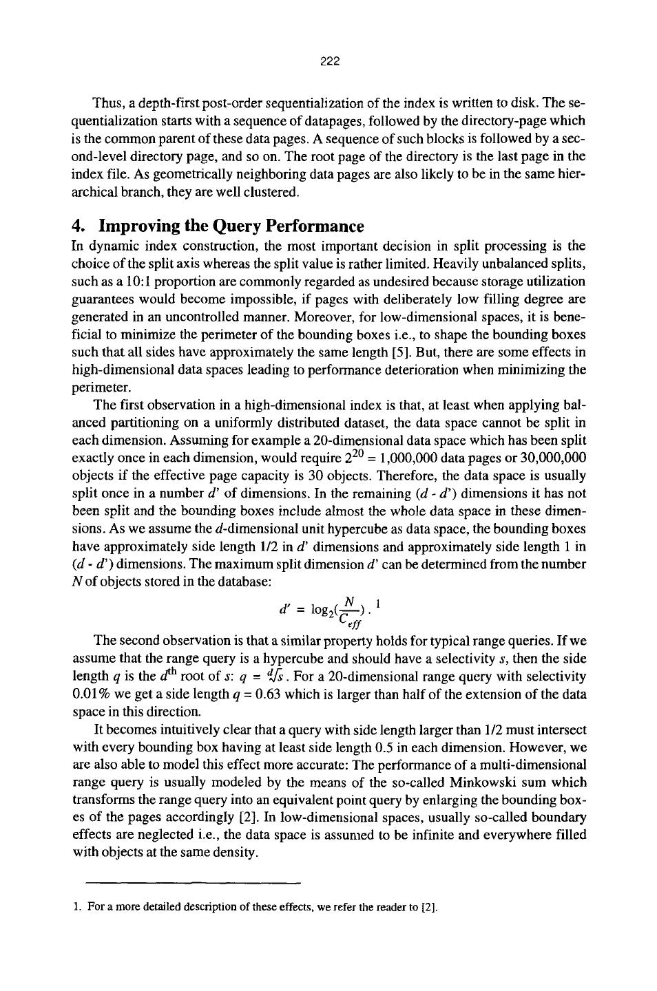
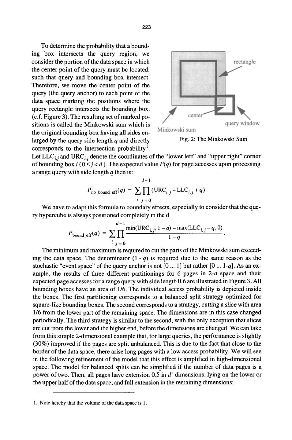
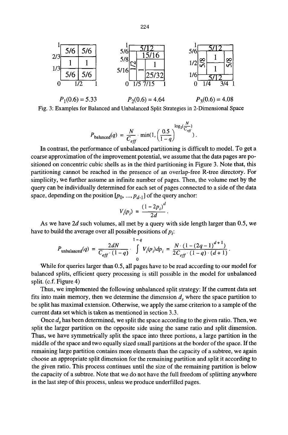
8 . 223 To determine the probability that a bound- ing box intersects the query region, we consider the portion of the data space in which the center point of the query must be located, such that query and bounding box intersect. Therefore, we move the center point of the query (the query anchor) to each point of the data space marking the positions where the query rectangle intersects the bounding box. (c.f. Figure 3). The resulting set of marked po- sitions is called the Minkowski sum which is the original bounding box having all sides en- larged by the query side length q and directly Fig. 2: The Minkowski Sum corresponds to the intersection probability 1. Let LLCi,j and URCi,j denote the coordinates of the "lower left" and "upper right" corner of bounding box i (0 < j < d ). The expected value P(q) for page accesses upon processing a range query with side length q then is: d-I Pno_bound_eff(q) = ~ H (URCi, j - LLCi, j + q) i j=0 We have to adapt this formula to boundary effects, especially to consider that the que- ry hypercube is always positioned completely in the d d-1 Pbound elf(q) = ~ I ' I min(URCi'j' 1 - q) - max(LLCi, j - q, 0) - 1-q i j=0 The minimum and maximum is required to cut the parts of the Minkowski sum exceed- ing the data space. The denominator (1 -q) is required due to the same reason as the stochastic "event space" of the query anchor is not [0 ... 1] but rather [0 ... I-q]. As an ex- ample, the results of three different partitionings for 6 pages in 2-d space and their expected page accesses for a range query with side length 0.6 are illustrated in Figure 3. All bounding boxes have an area of 1/6. The individual access probability is depicted inside the boxes. The first partitioning corresponds to a balanced split strategy optimized for square-like bounding boxes. The second corresponds to a strategy, cutting a slice with area 1/6 from the lower part of the remaining space. The dimensions are in this case changed periodically. The third strategy is similar to the second, with the only exception that slices are cut from the lower and the higher end, before the dimensions are changed. We can take from this simple 2-dimensional example that, for large queries, the performance is slightly (30%) improved if the pages are split unbalanced. This is due to the fact that close to the border of the data space, there arise long pages with a low access probability. We will see in the following refinement of the model that this effect is amplified in high-dimensional space. The model for balanced splits can be simplified if the number of data pages is a power of two. Then, all pages have extension 0.5 in d' dimensions, lying on the lower or the upper half of the data space, and full extension in the remaining dimensions: 1. Note hereby that the volume of the data space is 1. 

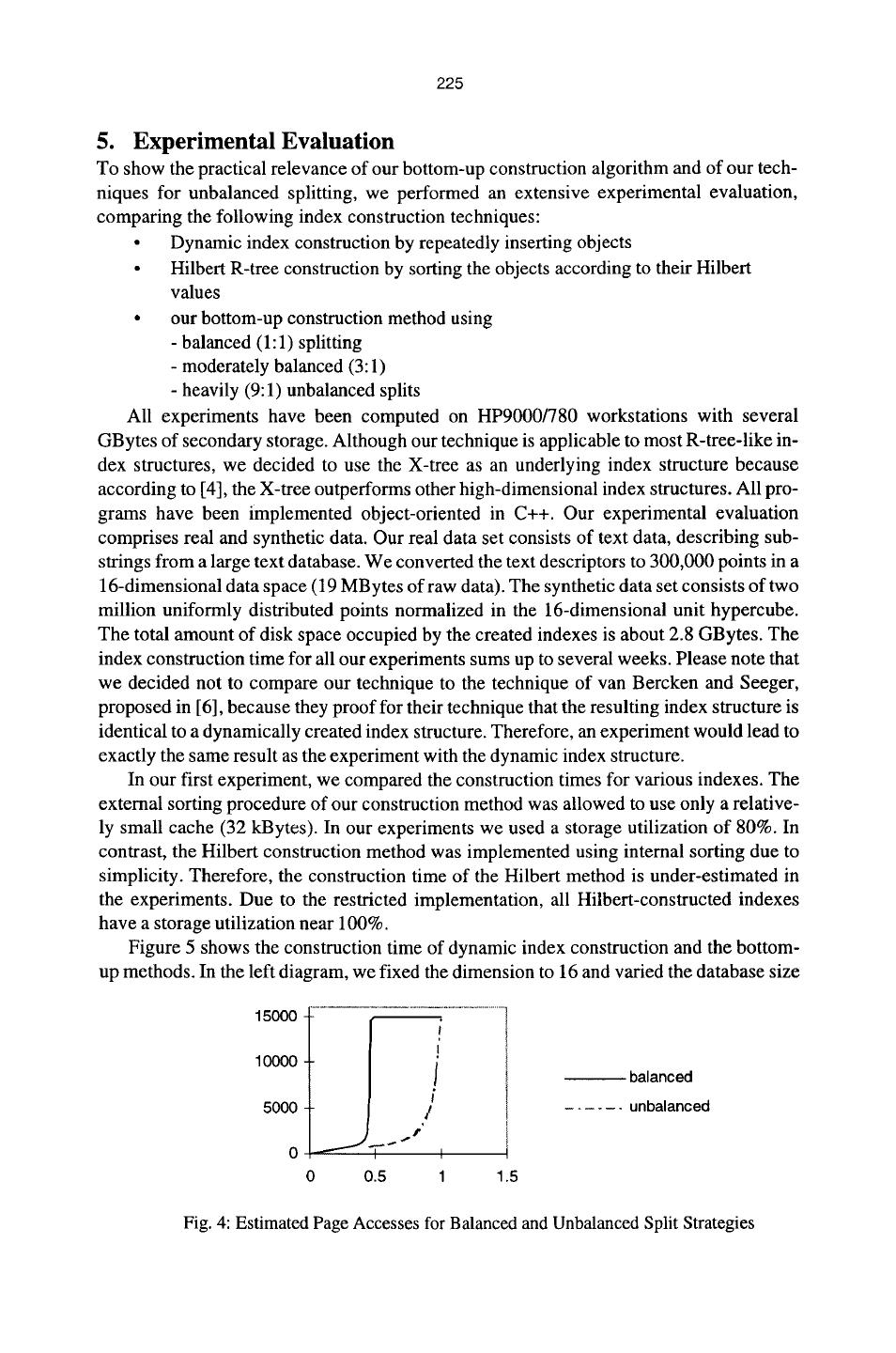
9 . 224 1 5/6 5/6 5/~ 5/12 5/1 5/12 2/3 5/8 15/16 1 1 ~ 1 1/2 "~ !~ 1/3 5/16 ~ " ' 1 5/6 5/6 25/32 1/6 5/12 0 1/2 1 0 1/5 7/15 0 1/4 3/4 1 Pt(0.6) = 5.33 P2(0.6) = 4.64 P3(0.6) = 4.08 Fig. 3: Examples for Balanced and Unbalanced Split Strategies in 2-Dimensional Space l~ Pbalanced(q) = Ceff In contrast, the performance of unbalanced partitioning is difficult to model. To get a coarse approximation of the improvement potential, we assume that the data pages are po- sitioned on concentric cubic shells as in the third partitioning in Figure 3. Note that, this partitioning cannot be reached in the presence of an overlap-free R-tree directory. For simplicity, we further assume an infinite number of pages. Then, the volume met by the query can be individually determined for each set of pages connected to a side of the data space, depending on the position [P0..... Pd-l] of the query anchor: (1 - 2Pi) d Vi(Pi) -- 2d As we have 2d such volumes, all met by a query with side length larger than 0.5, we have to build the average over all possible positions ofpi: 1-q 2dN N . (1 1)d+l) eunbalanced(q) = Ceff. (1 - q) S Vi(Pi)dPi = 2Ceff. -(1( 2-qq-) . (d+ 1) ' 0 While for queries larger than 0.5, all pages have to be read according to our model for balanced splits, efficient query processing is still possible in the model for unbalanced split. (c.f. Figure 4) Thus, we implemented the following unbalanced split strategy: If the current data set fits into main memory, then we determine the dimension d s where the space partition to be split has maximal extension. Otherwise, we apply the same criterion to a sample of the current data set which is taken as mentioned in section 3.3. Once d s has been determined, we split the space according to the given ratio. Then, we split the larger partition on the opposite side using the same ratio and split dimension. Thus, we have symmetrically split the space into three portions, a large partition in the middle of the space and two equally sized small partitions at the border of the space. If the remaining large partition contains more elements than the capacity of a subtree, we again choose an appropriate split dimension for the remaining partition and split it according to the given ratio. This process continues until the size of the remaining partition is below the capacity of a subtree. Note that we do not have the full freedom of splitting anywhere in the last step of this process, unless we produce underfilled pages. 

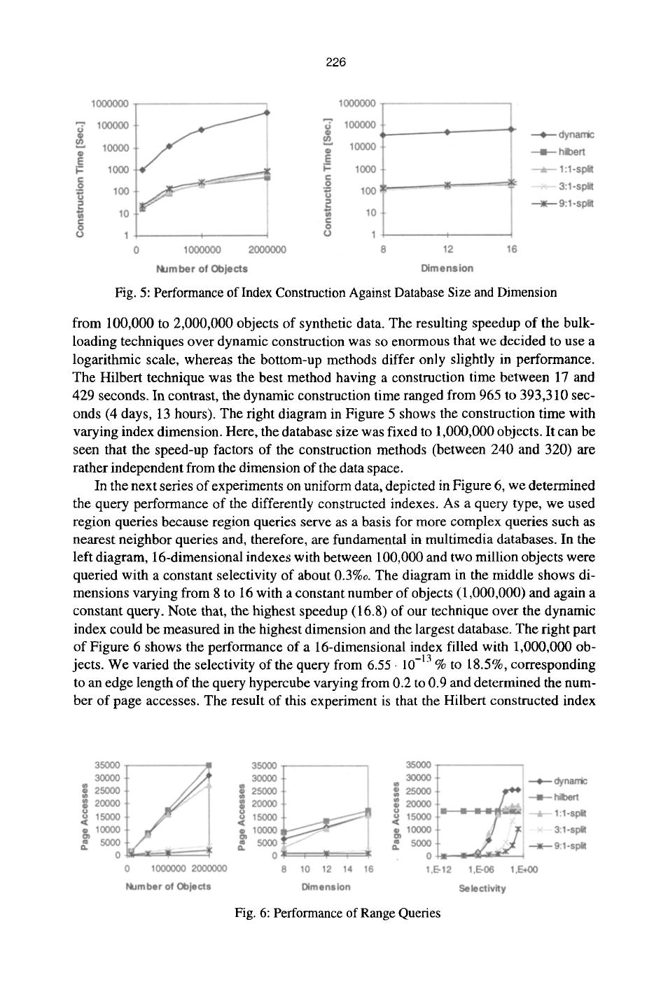
10 . 225 5. Experimental Evaluation To show the practical relevance of our bottom-up construction algorithm and of our tech- niques for unbalanced splitting, we performed an extensive experimental evaluation, comparing the following index construction techniques: 9 Dynamic index construction by repeatedly inserting objects 9 Hilbert R-tree construction by sorting the objects according to their Hilbert values 9 our bottom-up construction method using - balanced (1:1) splitting - moderately balanced (3:1) - heavily (9:1) unbalanced splits All experiments have been computed on HP9000/780 workstations with several GBytes of secondary storage. Although our technique is applicable to most R-tree-like in- dex structures, we decided to use the X-tree as an underlying index structure because according to [4], the X-tree outperforms other high-dimensional index structures. All pro- grams have been implemented object-oriented in C++. Our experimental evaluation comprises real and synthetic data. Our real data set consists of text data, describing sub- strings from a large text database. We converted the text descriptors to 300,000 points in a 16-dimensional data space (19 MBytes of raw data). The synthetic data set consists of two million uniformly distributed points normalized in the 16-dimensional unit hypercube. The total amount of disk space occupied by the created indexes is about 2.8 GBytes. The index construction time for all our experiments sums up to several weeks. Please note that we decided not to compare our technique to the technique of van Bercken and Seeger, proposed in [6], because they proof for their technique that the resulting index structure is identical to a dynamically created index structure. Therefore, an experiment would lead to exactly the same result as the experiment with the dynamic index structure. In our first experiment, we compared the construction times for various indexes. The external sorting procedure of our construction method was allowed to use only a relative- ly small cache (32 kBytes). In our experiments we used a storage utilization of 80%. In contrast, the Hilbert construction method was implemented using internal sorting due to simplicity. Therefore, the construction time of the Hilbert method is under-estimated in the experiments. Due to the restricted implementation, all Hilbert-constructed indexes have a storage utilization near 100%. Figure 5 shows the construction time of dynamic index construction and the bottom- 150o0 /,__ up methods. In the left diagram, we fixed the dimension to 16 and varied the database size !i 10000 / ~ balanced i 5000 / ...... unbalanced P 0 ', 0 0.5 1 1.5 Fig. 4: Estimated Page Accesses for Balanced and Unbalanced Split Strategies 

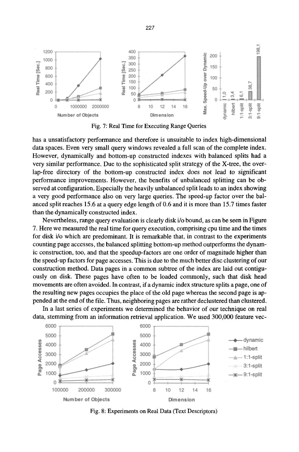
11 . 226 Fig. 5: Performance of Index Construction Against Database Size and Dimension from 100,000 to 2,000,000 objects of synthetic data. The resulting speedup of the bulk- loading techniques over dynamic construction was so enormous that we decided to use a logarithmic scale, whereas the bottom-up methods differ only slightly in performance. The Hilbert technique was the best method having a construction time between 17 and 429 seconds. In contrast, the dynamic construction time ranged from 965 to 393,310 sec- onds (4 days, 13 hours). The right diagram in Figure 5 shows the construction time with varying index dimension. Here, the database size was fixed to 1,000,000 objects. It can be seen that the speed-up factors of the construction methods (between 240 and 320) are rather independent from the dimension of the data space. In the next series of experiments on uniform data, depicted in Figure 6, we determined the query performance of the differently constructed indexes. As a query type, we used region queries because region queries serve as a basis for more complex queries such as nearest neighbor queries and, therefore, are fundamental in multimedia databases. In the left diagram, 16-dimensional indexes with between 100,000 and two million objects were queried with a constant selectivity of about 0.3%0. The diagram in the middle shows di- mensions varying from 8 to 16 with a constant number of objects (1,000,000) and again a constant query. Note that, the highest speedup (16.8) of our technique over the dynamic index could be measured in the highest dimension and the largest database. The right part of Figure 6 shows the performance of a 16-dimensional index filled with 1,000,000 ob- jects. We varied the selectivity of the query from 6.55 9 10-13 % to 18.5%, corresponding to an edge length of the query hypercube varying from 0.2 to 0.9 and determined the num- ber of page accesses. The result of this experiment is that the Hilbert constructed index Fig. 6: Performance of Range Queries 

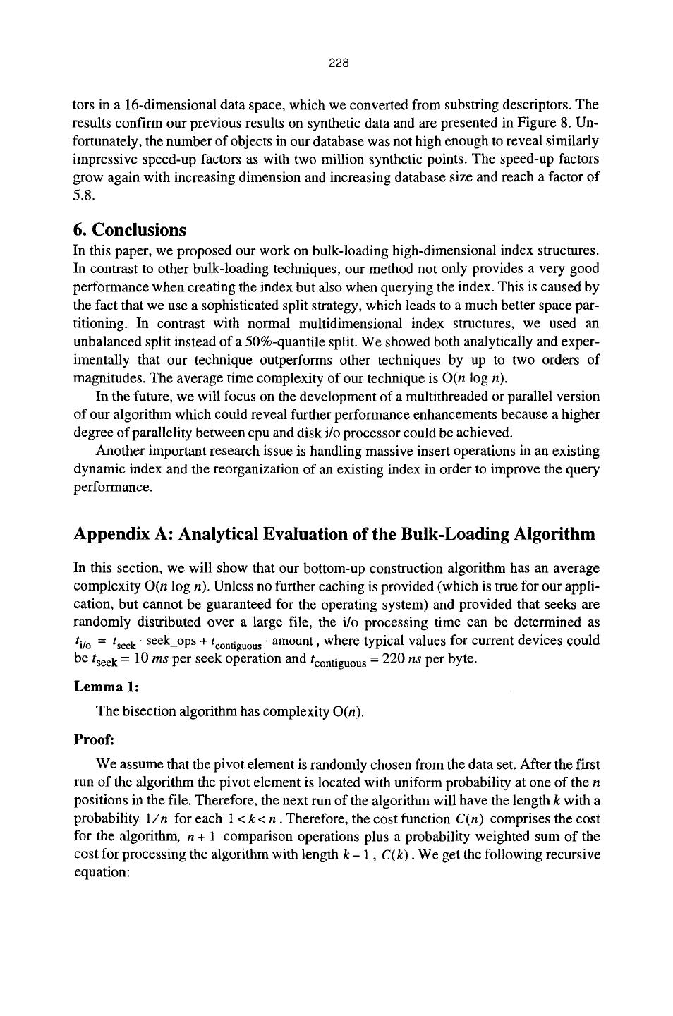
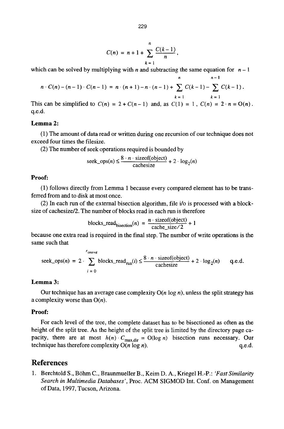
12 . 227 Fig. 7: Real Time for Executing Range Queries has a unsatisfactory performance and therefore is unsuitable to index high-dimensional data spaces. Even very small query windows revealed a full scan of the complete index. However, dynamically and bottom-up constructed indexes with balanced splits had a very similar performance. Due to the sophisticated split strategy of the X-tree, the over- lap-free directory of the bottom-up constructed index does not lead to significant performance improvements. However, the benefits of unbalanced splitting can be ob- served at configuration. Especially the heavily unbalanced split leads to an index showing a very good performance also on very large queries. The speed-up factor over the bal- anced split reaches 15.6 at a query edge length of 0.6 and it is more than 15.7 times faster than the dynamically constructed index. Nevertheless, range query evaluation is clearly disk i/o bound, as can be seen in Figure 7. Here we measured the real time for query execution, comprising cpu time and the times for disk i/o which are predominant. It is remarkable that, in contrast to the experiments counting page accesses, the balanced splitting bottom-up method outperforms the dynam- ic construction, too, and that the speedup-factors are one order of magnitude higher than the speed-up factors for page accesses. This is due to the much better disc clustering of our construction method. Data pages in a common subtree of the index are laid out contigu- ously on disk. These pages have often to be loaded commonly, such that disk head movements are often avoided. In contrast, if a dynamic index structure splits a page, one of the resulting new pages occupies the place of the old page whereas the second page is ap- pended at the end of the file. Thus, neighboring pages are rather declustered than clustered. In a last series of experiments we determined the behavior of our technique on real data, stemming from an information retrieval application. We used 300,000 feature vec- Fig. 8: Experiments on Real Data (Text Descriptors) 

13 . 228 tors in a 16-dimensional data space, which we converted from substring descriptors. The results confirm our previous results on synthetic data and are presented in Figure 8. Un- fortunately, the number of objects in our database was not high enough to reveal similarly impressive speed-up factors as with two million synthetic points. The speed-up factors grow again with increasing dimension and increasing database size and reach a factor of 5.8. 6. Conclusions In this paper, we proposed our work on bulk-loading high-dimensional index structures. In contrast to other bulk-loading techniques, our method not only provides a very good performance when creating the index but also when querying the index. This is caused by the fact that we use a sophisticated split strategy, which leads to a much better space par- titioning. In contrast with normal multidimensional index structures, we used an unbalanced split instead of a 50%-quantile split. We showed both analytically and exper- imentally that our technique outperforms other techniques by up to two orders of magnitudes. The average time complexity of our technique is O(n log n). In the future, we will focus on the development of a multithreaded or parallel version of our algorithm which could reveal further performance enhancements because a higher degree of parallelity between cpu and disk i/o processor could be achieved. Another important research issue is handling massive insert operations in an existing dynamic index and the reorganization of an existing index in order to improve the query performance. Appendix A: Analytical Evaluation of the Bulk-Loading Algorithm In this section, we will show that our bottom-up construction algorithm has an average complexity O(n log n). Unless no further caching is provided (which is true for our appli- cation, but cannot be guaranteed for the operating system) and provided that seeks are randomly distributed over a large file, the i/o processing time can be determined as ti/o = t s e e k " seek_ops + t c o n t i g u o u s 9 amount, where typical values for current devices could be tseek = 10 m s per seek operation and t c o n t i g u o u s = 220 ns per byte. L e m m a 1: The bisection algorithm has complexity O(n). Proof: We assume that the pivot element is randomly chosen from the data set. After the first run of the algorithm the pivot element is located with uniform probability at one of the n positions in the file. Therefore, the next run of the algorithm will have the length k with a probability 1 / n for each 1 < k < n. Therefore, the cost function C(n) comprises the cost for the algorithm, n + 1 comparison operations plus a probability weighted sum of the cost for processing the algorithm with length k - 1, C ( k ) . We get the following recursive equation: 

14 . 229 ?1 C(n) = n + l + Z C(k-1) rl k=l which can be solved by multiplying with n and subtracting the same equation for n - 1 n n-1 n.C(n)-(n-1).C(n-1) = n.(n+l)-n.(n-1)+ Z C(k- 1)- Z C(k-1). k=l k=l This can be simplified to C(n) = 2 + C ( n - 1 and, as C(1) = 1, C(n) = 2. n = O(n). q.e.d. Lemma 2: (1) The amount of data read or written during one recursion of our technique does not exceed four times the filesize. (2) The number of seek operations required is bounded by seek_ops(n) < 8. n. sizeof(object) - cachesize + 2. log2(n) Proof: (1) follows directly from Lemma 1 because every compared element has to be trans- ferred from and to disk at most once. (2) In each run of the external bisection algorithm, file i/o is processed with a block- size of cachesize/2. The number of blocks read in each run is therefore blocks_readbisection(n) = n.cache_size/2Sizeof(object) +1 because one extra read is required in the final step. The number of write operations is the same such that rinterval seek ops(n) = 2. ~ blocks readrun(i) < 8. n. sizeof(object) + 2- log2(n) q.e.d. - - - cachesize i=0 Lemma 3: Our technique has an average case complexity O(n log n), unless the split strategy has a complexity worse than O(n). Proof: For each level of the tree, the complete dataset has to be bisectioned as often as the height of the split tree. As the height of the split tree is limited by the directory page ca- pacity, there are at most h(n).Cmax.di r = O(log n) bisection runs necessary. Our technique has therefore complexity O(n log n). q.e.d. References 1. Berchtold S., B6hm C., Braunmueller B., Keim D. A., Kriegel H.-P.: 'Fast Similarity Search in Multimedia Databases', Proc. A C M SIGMOD Int. Conf. on Management of Data, 1997, Tucson, Arizona. 

15 . 230 2. Berchtold S., B6hm C., Keim D., Kriegel H.-P.: 'A CostModel For Nearest Neighbor Search in High-Dimensional Data Space', ACM PODS Symposium on Pricinples of Database Systems, Tucson, Arizona, 1997, SIGMOD BEST PAPER AWARD. 3. Berchtold S., Kriegel H.-P.: '$3: Similarity Search in CAD Database Systems', Proc. ACM SIGMOD Int. Conf. on Management of Data, 1997, Tucson, Arizona. 4. Berchtold S., Keim D., Kriegel H.-P.: 'The X-tree: An Index Structure for High- Dimensional Data', 22nd Conf. on Very Large Databases, 1996, Bombay, India, pp. 28-39. 5. Beckmann N., Kriegel H.-P., Schneider R., Seeger B.: 'The R*-tree: An Efficient and Robust Access Method for Points and Rectangles', Proc. ACM SIGMOD Int. Conf. on Management of Data, Atlantic City, NJ, 1990, pp. 322-331. 6. van den Bercken J., Seeger B., Widmayer P.:, 'A General Approach to Bulk Loading Multidimensional Index Structures', 23rd Conf. on Very Large Databases, 1997, Athens, Greece. 7. Faloutsos C., Barber R., Flickner M., Hafner J., et al.: 'Efficient and Effective Querying by Image Content', Journal of Intelligent Information Systems, 1994, Vol. 3, pp. 231-262. 8. Friedman J. H., Bentley J. L., Finkel R. A.: 'An Algorithm for Finding Best Matches in Logarithmic Expected Time', ACM Transactions on Mathematical Software, Vol. 3, No. 3, September 1977, pp. 209-226. 9. C.A.R. Hoare, 'Quicksort', Computer Journal, Vol. 5, No. 1, 1962. 10. Jagadish H. V.: 'A Retrieval Technique for Similar Shapes', Proc. ACM SIGMOD Int. Conf. on Management of Data, 1991, pp. 208-217. 11. Jain R, White D.A.: 'Similarity Indexing: Algorithms and Performance', Proc. SPIE Storage and Retrieval for Image and Video Databases IV, Vol. 2670, San Jose, CA, 1996, pp. 62-75. 12. Kamel I., Faloutsos C.: 'Hilbert R-tree: An Improved R-tree using Fractals'. Proc. 20th Int. Conf. on Very Large Databases (VLDB 94), pp. 500-509 13. Katayama N., Satoh S.: 'The SR-tree: An Index Structure for High-Dimensional Nearest Neighbor Queries', Proc. ACM SIGMOD Int. Conf. on Management of Data, 1997. 14. Lin K., Jagadish H. V., Faloutsos C.: 'The TV-tree: An Index Structure for High- Dimensional Data', VLDB Journal, Vol. 3, pp. 517-542, 1995. 15. Mehrotra R., Gary J.: 'Feature-Based Retrieval of Similar Shapes', Proc. 9th Int. Conf. on Data Engeneering, April 1993 16. Robinson J. T.: "The K-D-B-tree: A Search Structure for Large Multidimensional Dynamic Indexes', Proc. ACM SIGMOD Int. Conf. on Management of Data, 1981, pp. 10-18. 17. R. Sedgewick: 'Quicksort', Garland, New York, 1978. 18. Seidl T., Kriegel H.-P.: 'Efficient User-Adaptable Similarity Search in Large Multimedia Databases', Proc. 23rd Int. Conf. on Very Large Databases (VLDB~)7), Athens, Greece, 1997. 19. White D.A., Jain R.: 'Similarity indexing with the SS-tree', Proc. 12th Int. Conf on Data Engineering, New Orleans, LA, 1996.