datamining lect9

1 .DATA MINING LECTURE 8 Dimensionality Reduction PCA -- SVD

2 .The curse of dimensionality Real data usually have thousands , or millions of dimensions E.g., web documents, where the dimensionality is the vocabulary of words Facebook graph, where the dimensionality is the number of users Huge number of dimensions causes problems Data becomes very sparse , some algorithms become meaningless (e.g. density based clustering) The complexity of several algorithms depends on the dimensionality and they become infeasible.

3 .Dimensionality Reduction U sually the data can be described with fewer dimensions, without losing much of the meaning of the data. The data reside in a space of lower dimensionality Essentially, we assume that some of the data is noise, and we can approximate the useful part with a lower dimensionality space. Dimensionality reduction does not just reduce the amount of data, it often brings out the useful part of the data

4 .Dimensionality Reduction We have already seen a form of dimensionality reduction LSH, and random projections reduce the dimension while preserving the distances

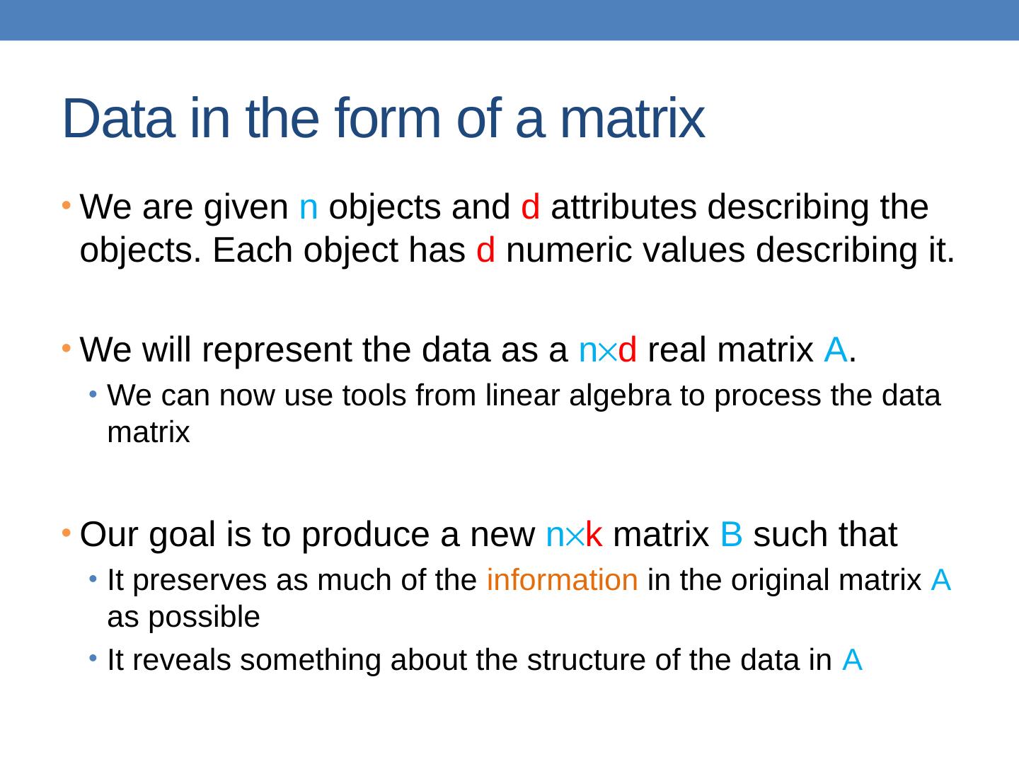
5 .Data in the form of a matrix We are given n objects and d attributes describing the objects. Each object has d numeric values describing it . We will represent the data as a n  d real matrix A . We can now use tools from linear algebra to process the data matrix Our goal is to produce a new n  k matrix B such that It preserves as much of the information in the original matrix A as possible It reveals something about the structure of the data in A

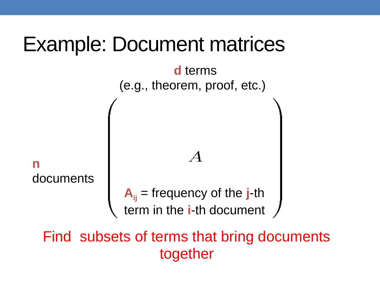
6 .Example: Document matrices n documents d terms (e.g., theorem, proof, etc.) A ij = frequency of the j -th term in the i -th document Find subsets of terms that bring documents together

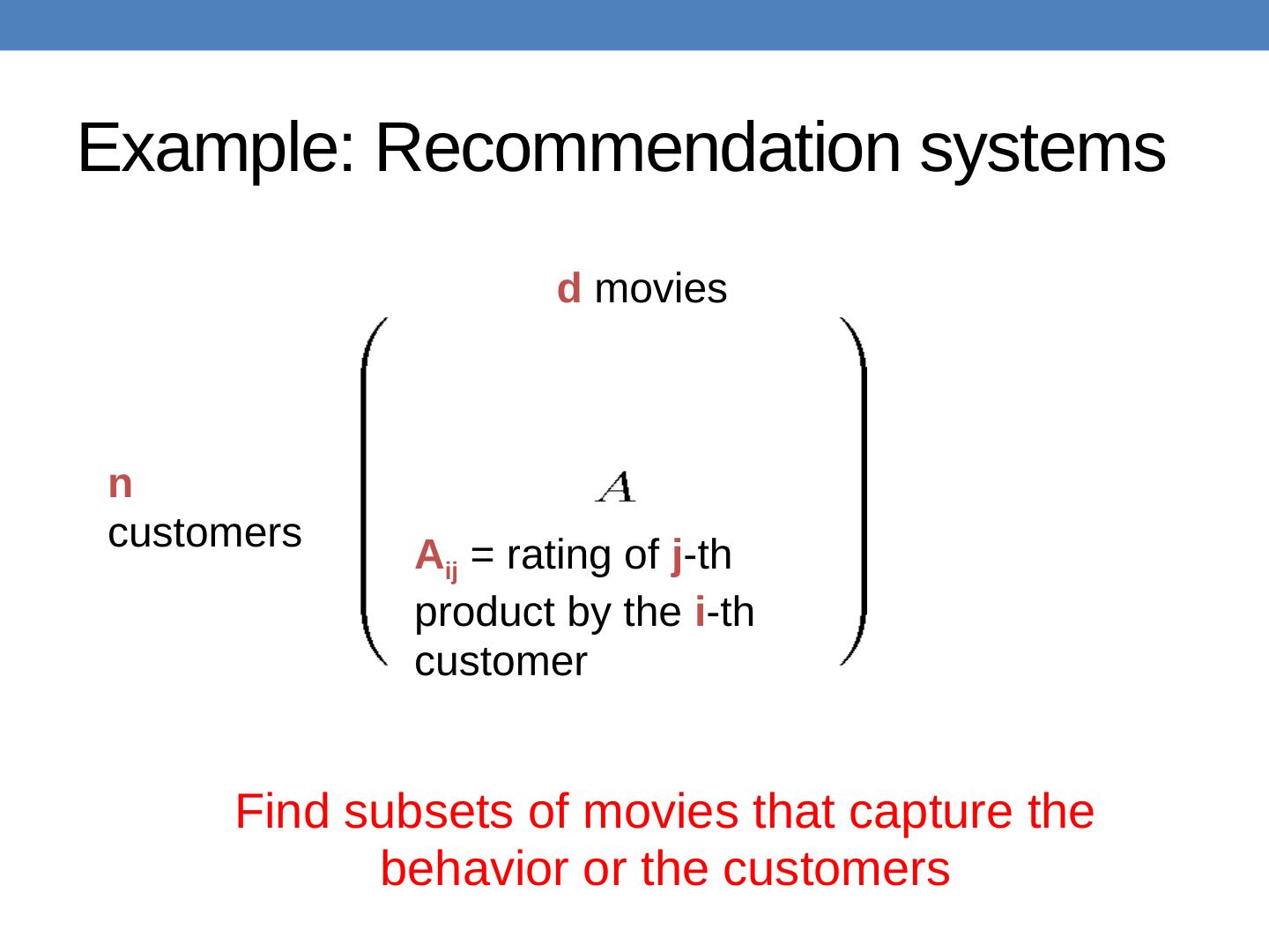
7 .Example: Recommendation systems n customers d movies A ij = rating of j - th product by the i - th customer Find subsets of movies that capture the behavior or the customers

8 .Linear algebra We assume that vectors are column vectors . We use for the transpose of vector ( row vector ) Dot product : ( ) The dot product is the projection of vector on (and vice versa) If (unit vector) then is the projection length of on orthogonal vectors Orthonormal vectors: two unit vectors that are orthogonal  

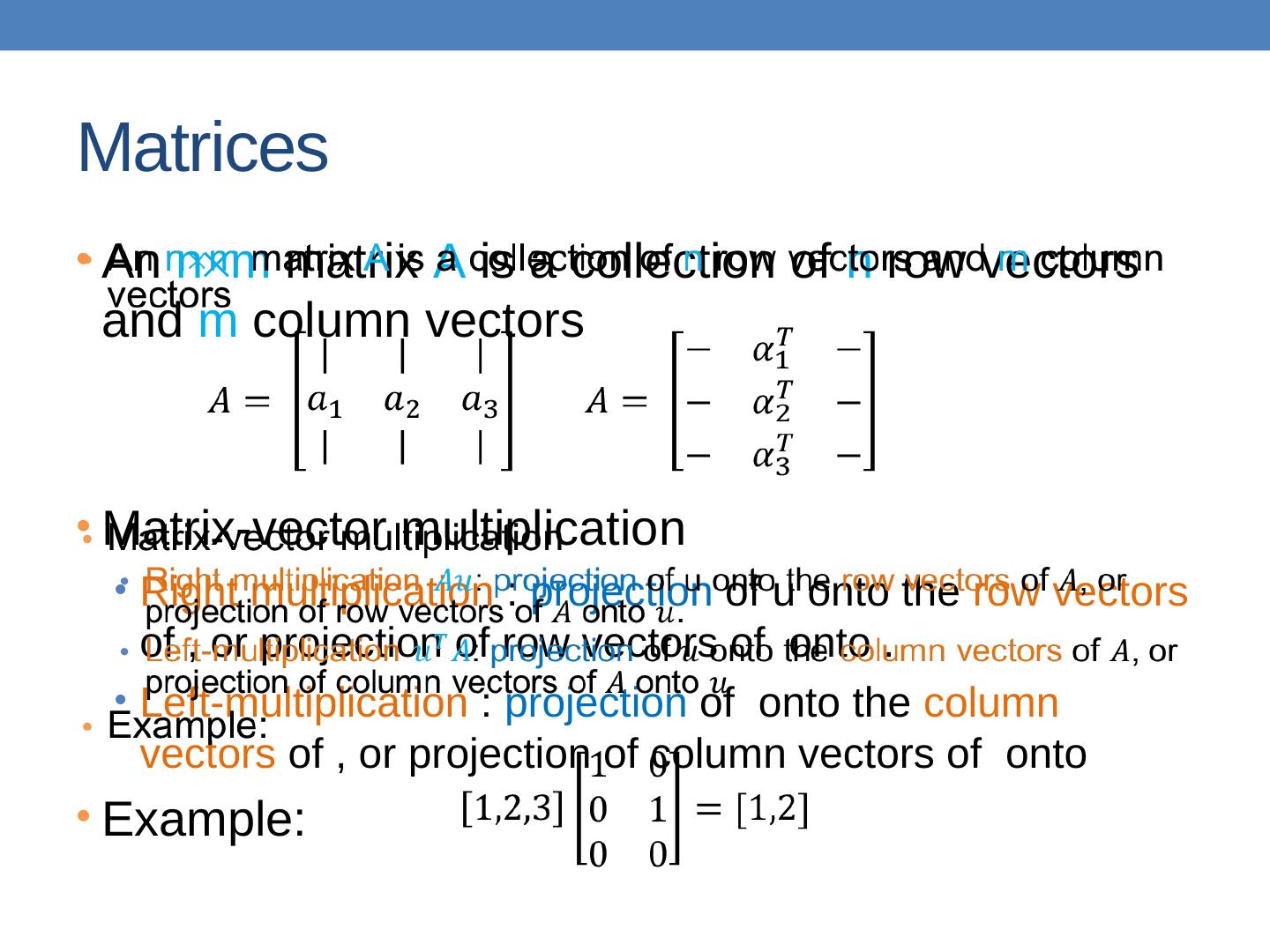
9 .Matrices An n m matrix A is a collection of n row vectors and m column vectors Matrix-vector multiplication Right multiplication : projection of u onto the row vectors of , or projection of row vectors of onto . Left-multiplication : projection of onto the column vectors of , or projection of column vectors of onto Example:  

10 .Rank Row space of A: The set of vectors that can be written as a linear combination of the rows of A All vectors of the form Column space of A: The set of vectors that can be written as a linear combination of the columns of A All vectors of the form Rank of A: the number of linearly independent row (or column) vectors These vectors define a basis for the row (or column) space of A  

11 .Rank-1 matrices In a rank-1 matrix, all columns (or rows) are multiples of the same column (or row) vector All rows are multiples of All columns are multiples of External product : ( ) The resulting has rank 1: all rows (or columns) are linearly dependent  

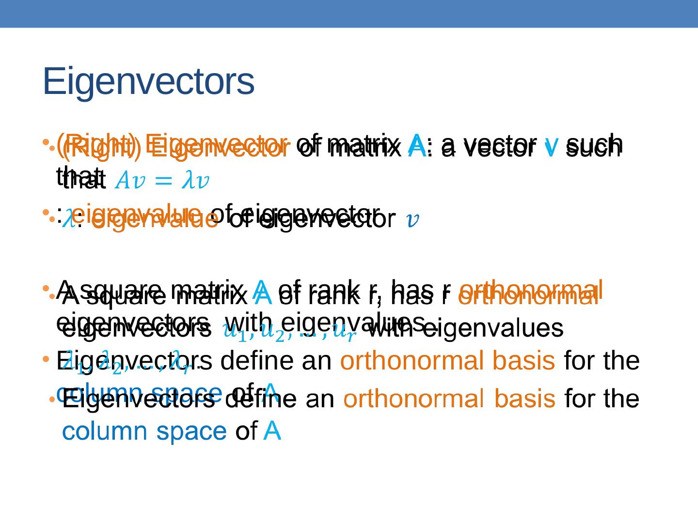
12 .Eigenvectors (Right) Eigenvector of matrix A : a vector v such that : eigenvalue of eigenvector A square matrix A of rank r, has r orthonormal eigenvectors with eigenvalues . Eigenvectors define an orthonormal basis for the column space of A  

13 .Singular Value Decomposition : singular values of matrix (also, the square roots of eigenvalues of and ) : left singular vectors of (also eigenvectors of ) : right singular vectors of (also, eigenvectors of )   [ n ×r ] [ r ×r ] [ r ×m ] r : rank of matrix A [ n ×m ] =

14 .Symmetric matrices Special case: A is symmetric positive definite matrix : Eigenvalues of A : Eigenvectors of A  

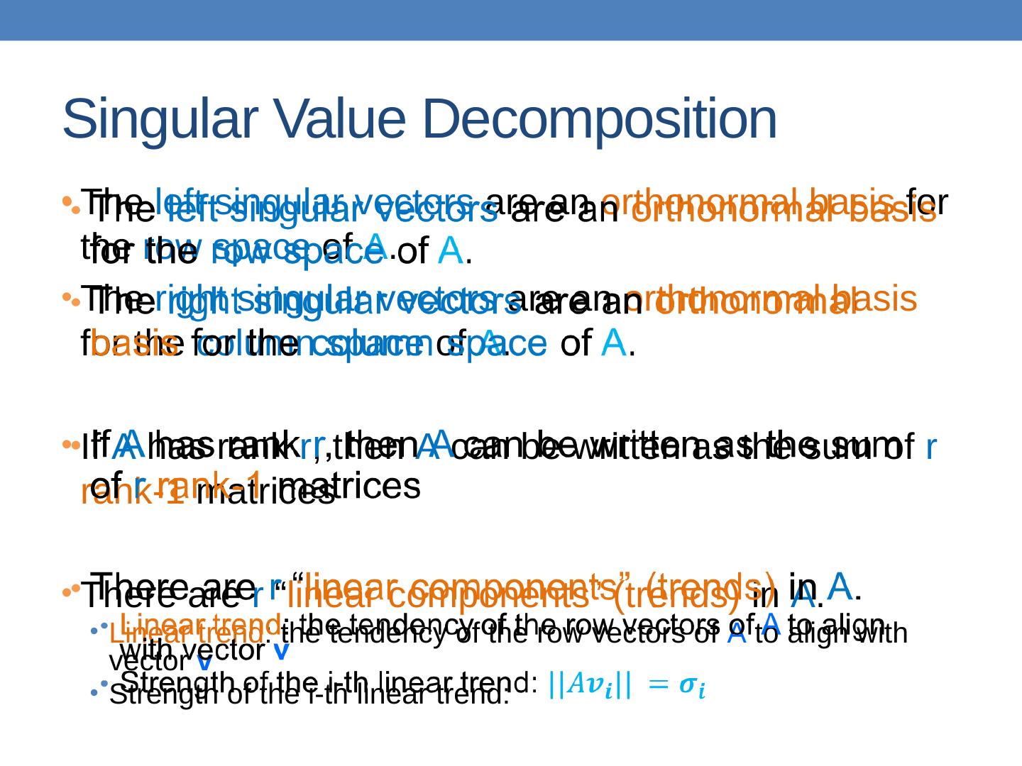
15 .Singular V alue D ecomposition The left singular vectors are an orthonormal basis for the row space of A . The right singular vectors are an orthonormal basis for the column space of A . If A has rank r , then A can be written as the sum of r rank-1 matrices There are r “ linear components” (trends) in A . Linear trend : the tendency of the row vectors of A to align with vector v Strength of the i- th linear trend:  

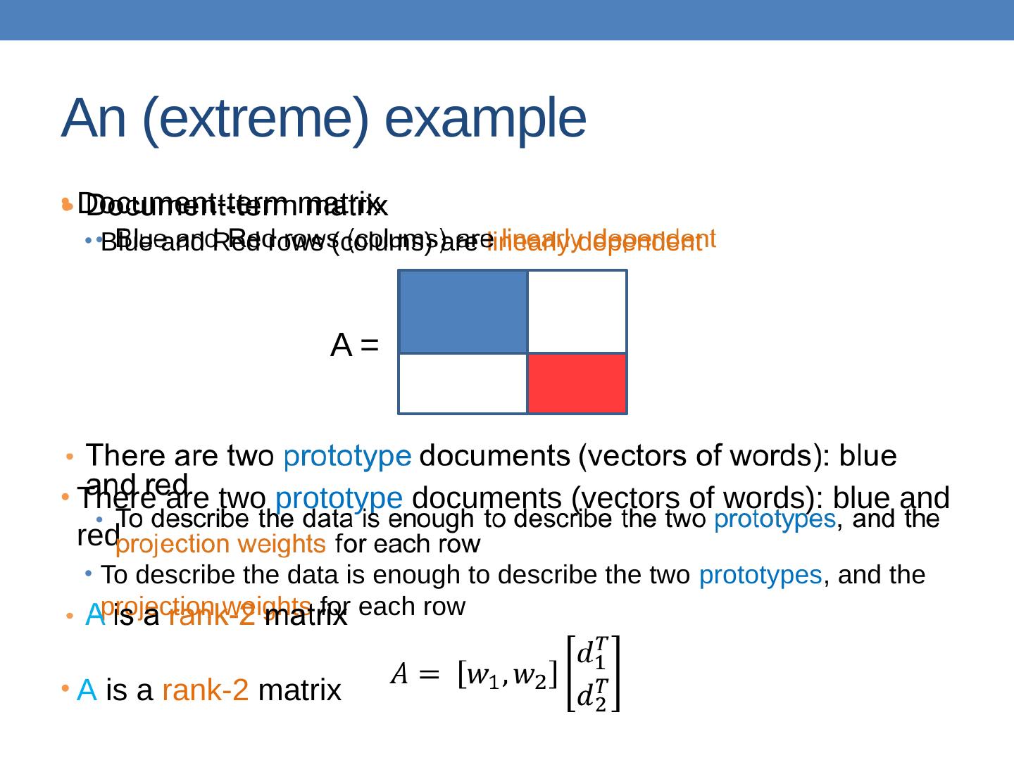
16 .An (extreme) example Document-term matrix Blue and Red rows ( colums ) are linearly dependent There are two prototype documents (vectors of words): blue and red To describe the data is enough to describe the two prototypes , and the projection weights for each row A is a rank-2 matrix   A =

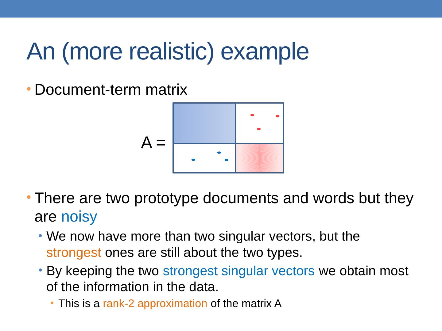
17 .An (more realistic) example Document-term matrix There are two prototype documents and words but they are noisy We now have more than two singular vectors, but the strongest ones are still about the two types. By keeping the two strongest singular vectors we obtain most of the information in the data. This is a rank-2 approximation of the matrix A A =

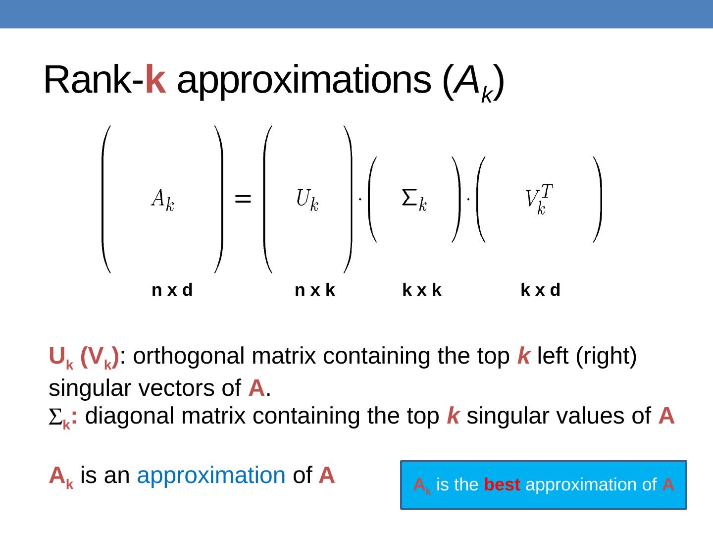
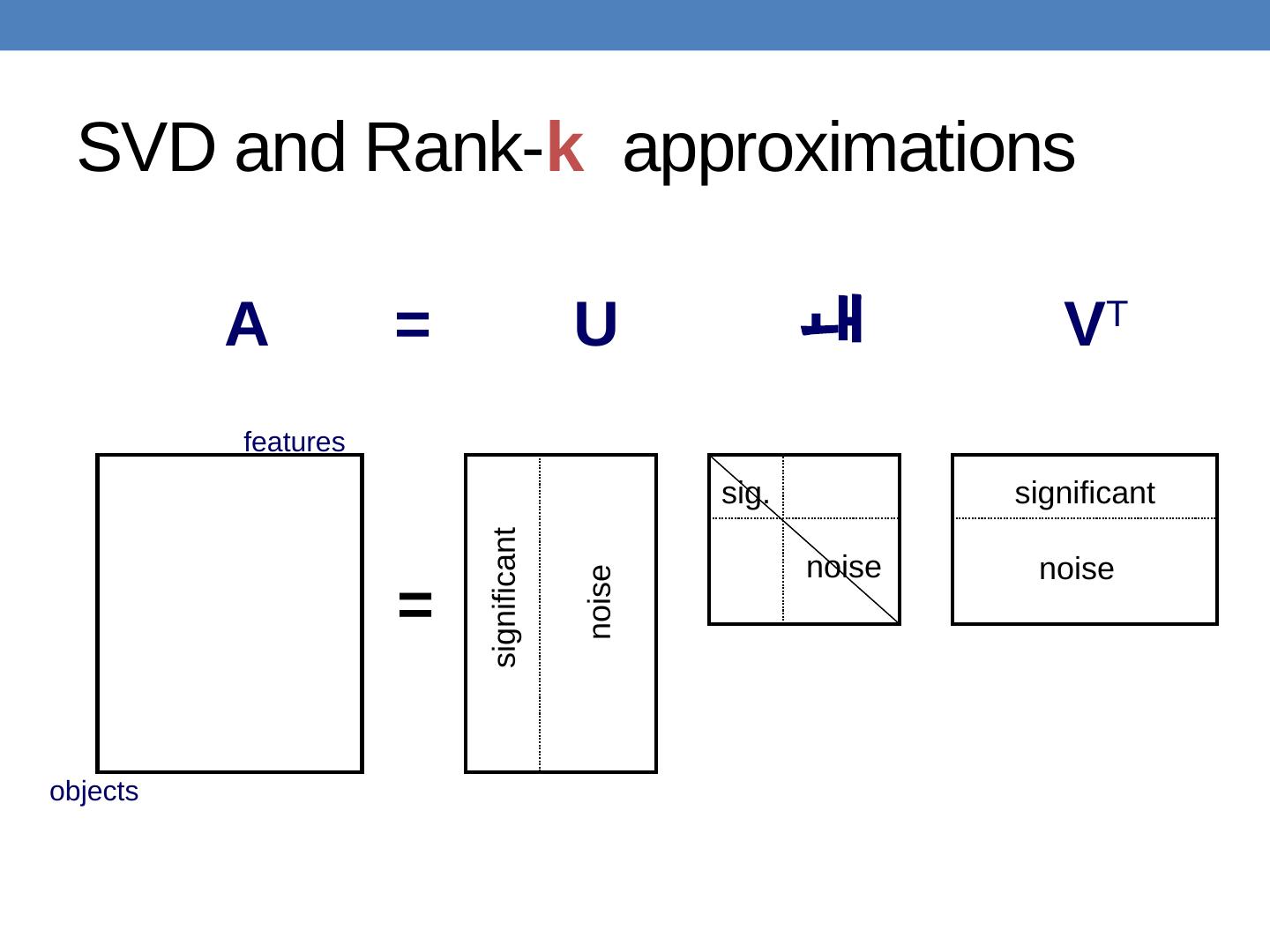
18 .Rank- k approximations ( A k ) U k ( V k ) : orthogonal matrix containing the top k left (right) singular vectors of A . k : diagonal matrix containing the top k singular values of A A k is an approximation of A n x d n x k k x k k x d A k is the best approximation of A

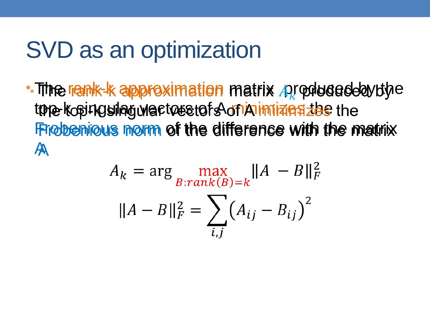
19 .SVD as an optimization The rank-k approximation matrix produced by the top-k singular vectors of A minimizes the Frobenious norm of the difference with the matrix A  

20 .What does this mean? We can project the row (and column) vectors of the matrix A into a k-dimensional space and preserve most of the information ( Ideally ) The k dimensions reveal latent features/aspects/topics of the term (document) space. ( Ideally ) The approximation of matrix A, contains all the useful information , and what is discarded is noise  

21 .Latent factor model Rows (columns) are linear combinations of k latent factors E.g., in our extreme document example there are two factors Some noise is added to this rank-k matrix resulting in higher rank SVD retrieves the latent factors (hopefully).

22 .A V T  U = objects features significant noise noise noise significant sig. = SVD and Rank- k approximations

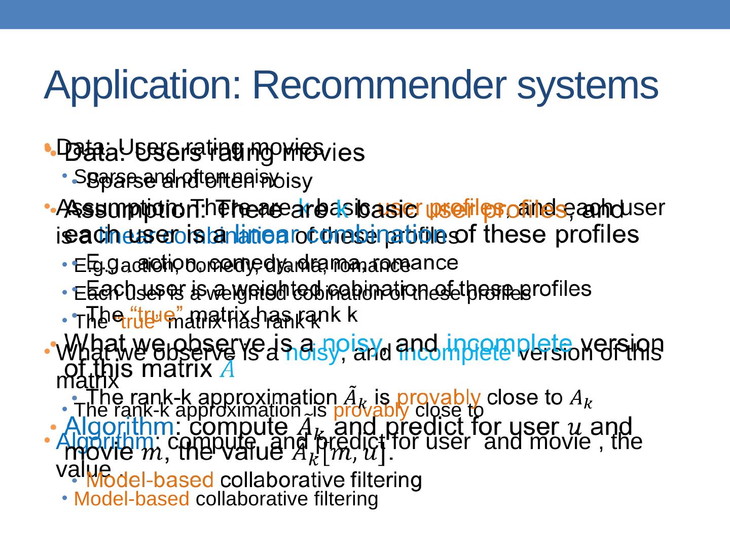
23 .Application: Recommender systems Data: Users rating movies Sparse and often noisy Assumption: There are k basic user profiles , and each user is a linear combination of these profiles E.g., action, comedy, drama, romance Each user is a weighted cobination of these profiles The “true” matrix has rank k What we observe is a noisy , and incomplete version of this matrix The rank-k approximation is provably close to Algorithm : compute and predict for user and movie , the value . Model-based collaborative filtering  

24 .SVD and PCA PCA is a special case of SVD on the centered covariance matrix .

25 .Covariance matrix Goal: reduce the dimensionality while preserving the “ information in the data” Information in the data: variability in the data We measure variability using the covariance matrix . Sample covariance of variables X and Y Given matrix A , remove the mean of each column from the column vectors to get the centered matrix C The matrix is the covariance matrix of the row vectors of A .  

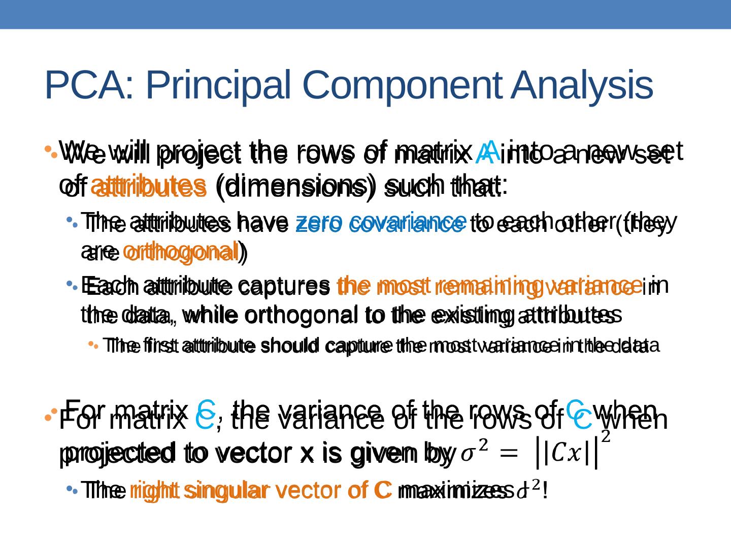
26 .PCA: Principal Component Analysis We will project the rows of matrix A into a new set of attributes (dimensions) such that: The attributes have zero covariance to each other (they are orthogonal ) Each attribute captures the most remaining variance in the data, while orthogonal to the existing attributes The first attribute should capture the most variance in the data For matrix C , the variance of the rows of C when projected to vector x is given by The right singular vector of C maximizes !  

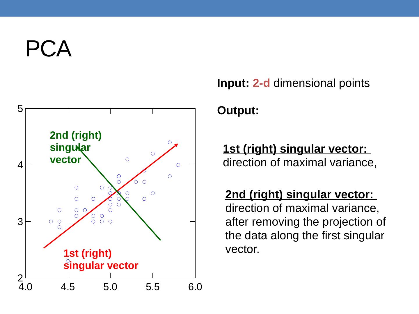
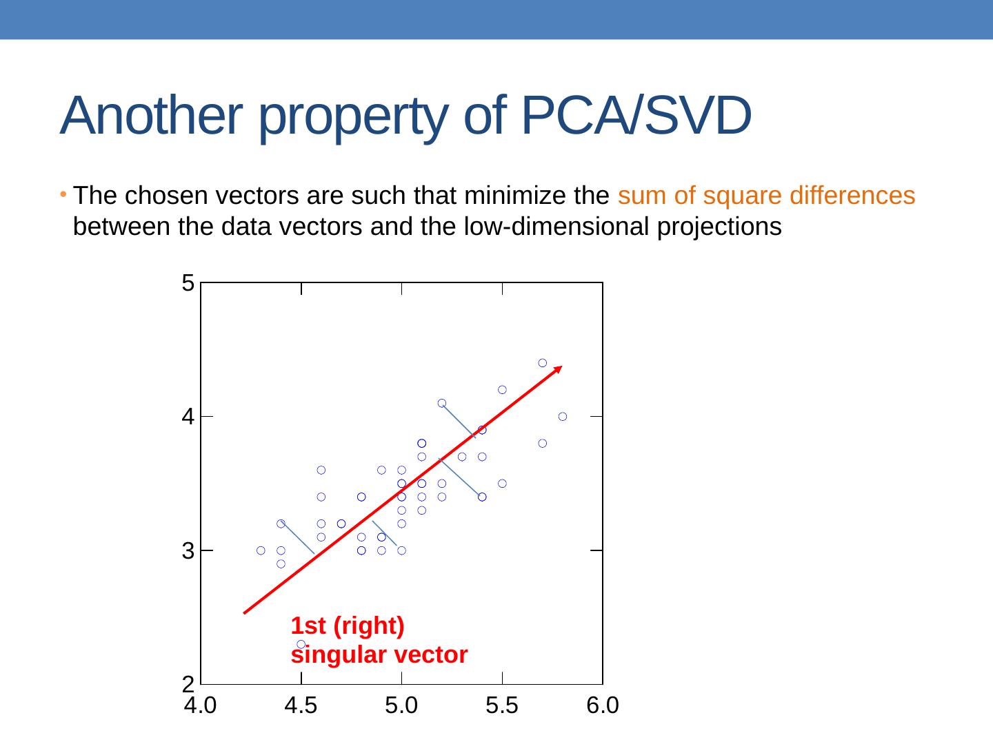
27 .PCA Input: 2-d dimensional points Output: 1st (right) singular vector 1st (right) singular vector: direction of maximal variance, 2nd (right) singular vector 2nd (right) singular vector: direction of maximal variance, after removing the projection of the data along the first singular vector.

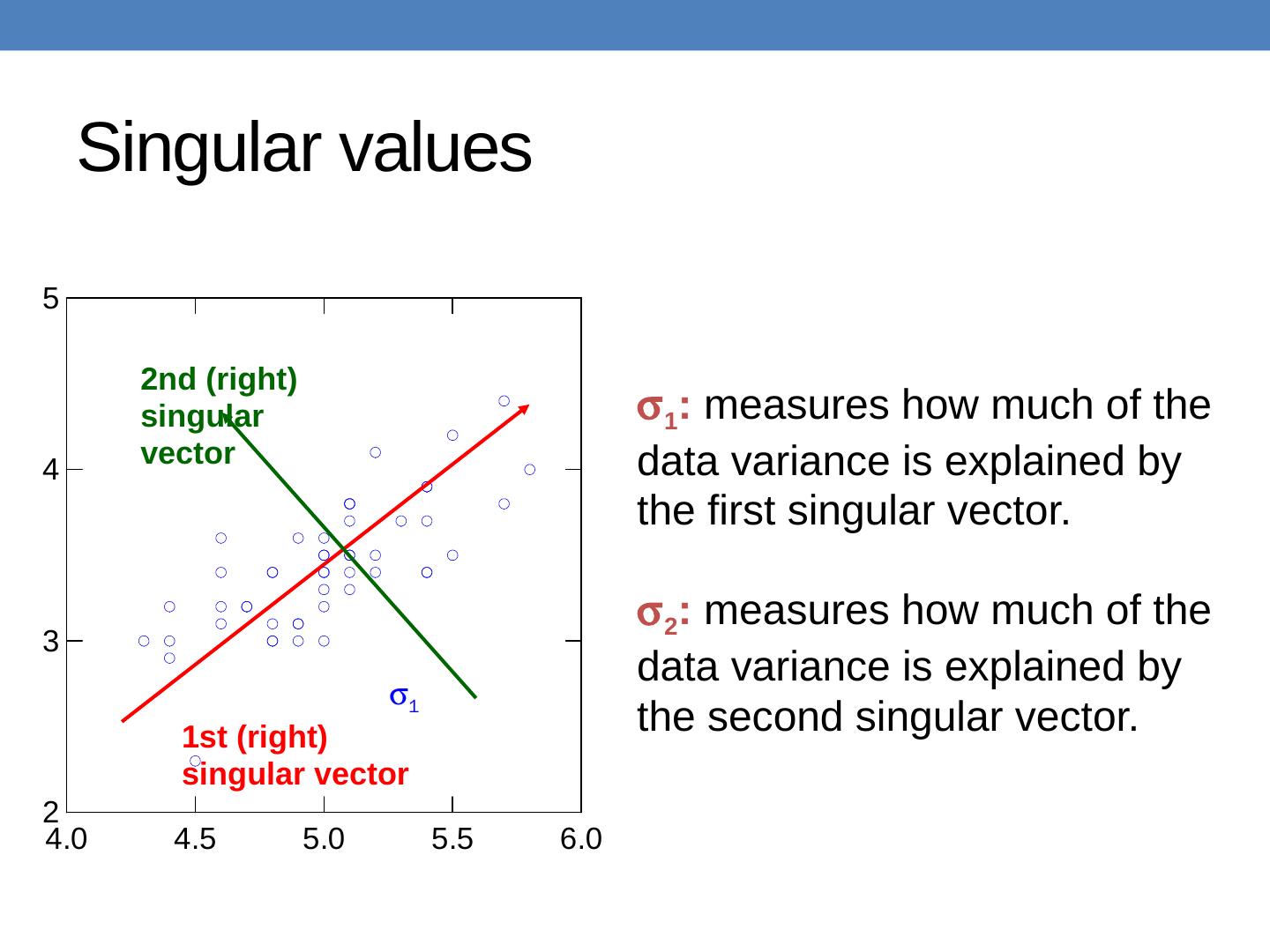
28 .Singular values  1 : measures how much of the data variance is explained by the first singular vector.  2 : measures how much of the data variance is explained by the second singular vector.  1 1st (right) singular vector 2nd (right) singular vector

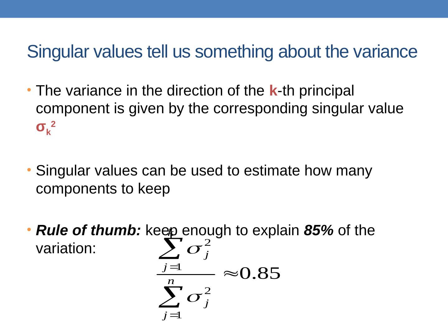
29 .Singular values tell us something about the variance The variance in the direction of the k -th principal component is given by the corresponding singular value σ k 2 Singular values can be used to estimate how many components to keep Rule of thumb: keep enough to explain 85% of the variation: