拟合和对齐

1 .Fitting and Alignment Computer Vision Jia-Bin Huang, Virginia Tech Many slides from S. Lazebnik and D. Hoiem

2 .Administrative Stuffs Homework grading policy Graduate students: graded out of 600 points Undergrad students: graded out of 525 points For example, grad students need to complete on average 25 points extra credits. HW 1 Extra credits due 11:59 PM Friday 9/23 Competition: Edge Detection Submission link Leaderboard Anonymous feedback Lectures are too fast, too many slides

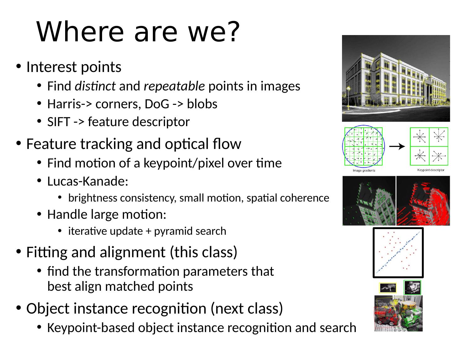
3 .Where are we? Interest points Find distinct and repeatable points in images Harris-> corners, DoG -> blobs SIFT -> feature descriptor Feature tracking and optical flow Find motion of a keypoint /pixel over time Lucas- Kanade : brightness consistency, small motion, spatial coherence Handle large motion: iterative update + pyramid search Fitting and alignment (this class) find the transformation parameters that best align matched points Object instance recognition (next class) Keypoint -based object instance recognition and search

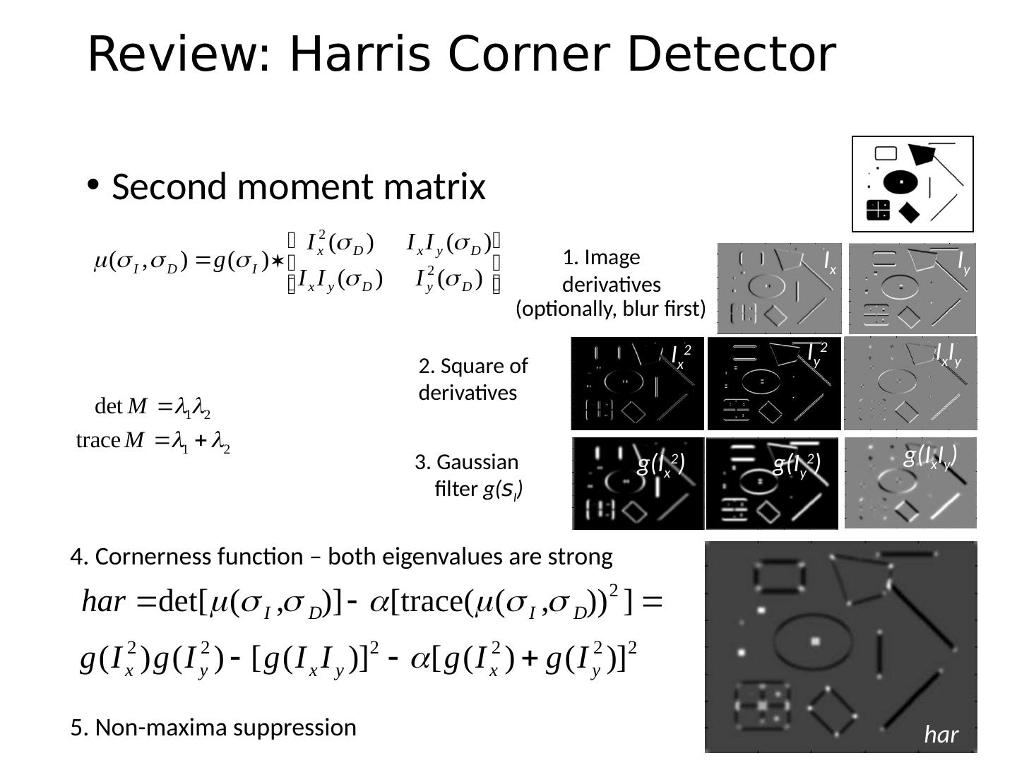
4 .Review: Harris Corner Detector Second moment matrix 4 1. Image derivatives 2. Square of derivatives 3. Gaussian filter g( s I ) I x I y I x 2 I y 2 I x I y g(I x 2 ) g(I y 2 ) g(I x I y ) 4. Cornerness function – both eigenvalues are strong har 5. Non-maxima suppression (optionally, blur first)

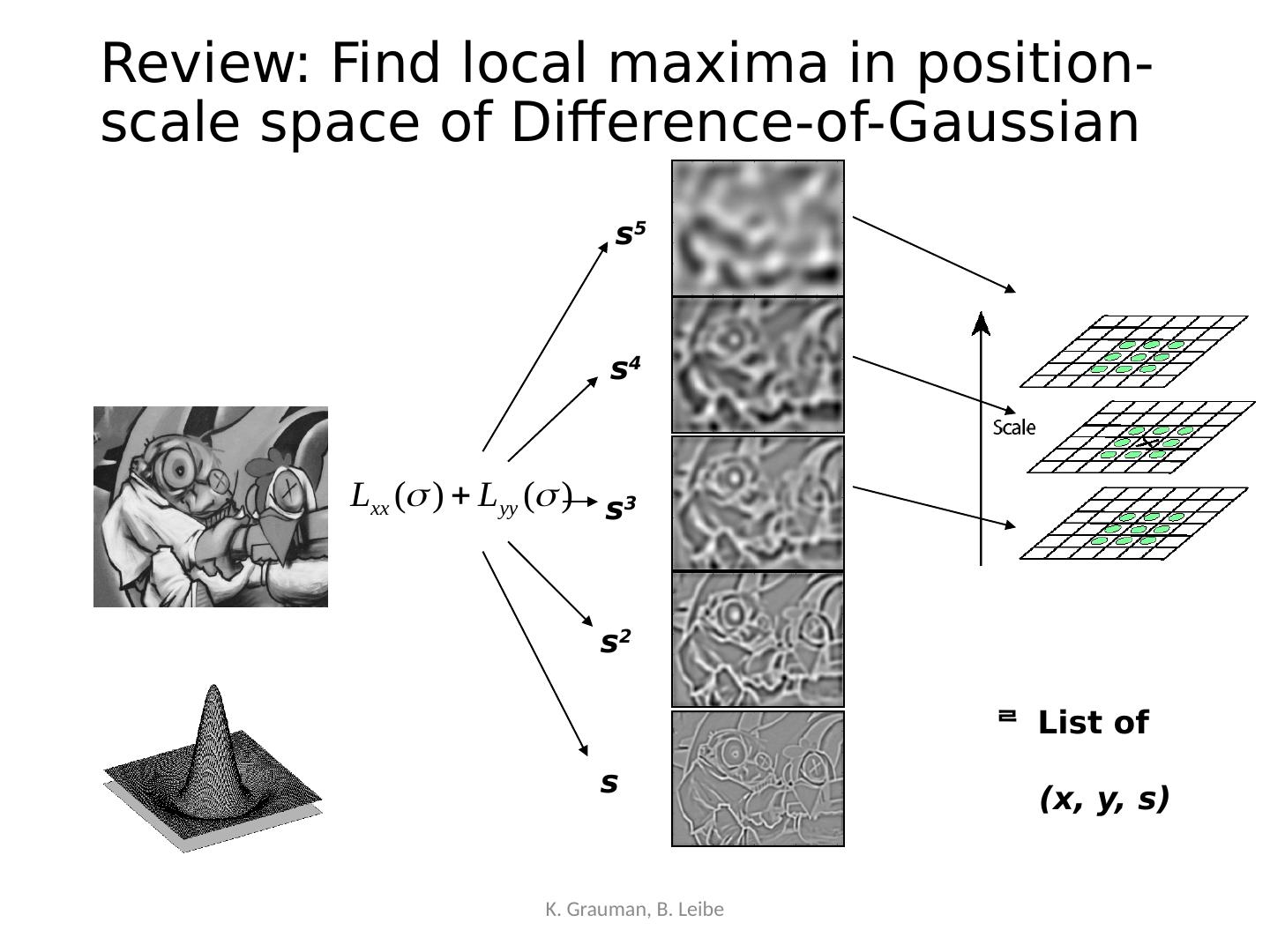
5 .Review: Find local maxima in position-scale space of Difference-of-Gaussian K. Grauman, B. Leibe s s 2 s 3 s 4 s 5  L ist of (x, y, s)

6 .Review: SIFT Descriptor [Lowe, ICCV 1999] Histogram of oriented gradients Captures important texture information Robust to small translations / affine deformations K. Grauman, B. Leibe

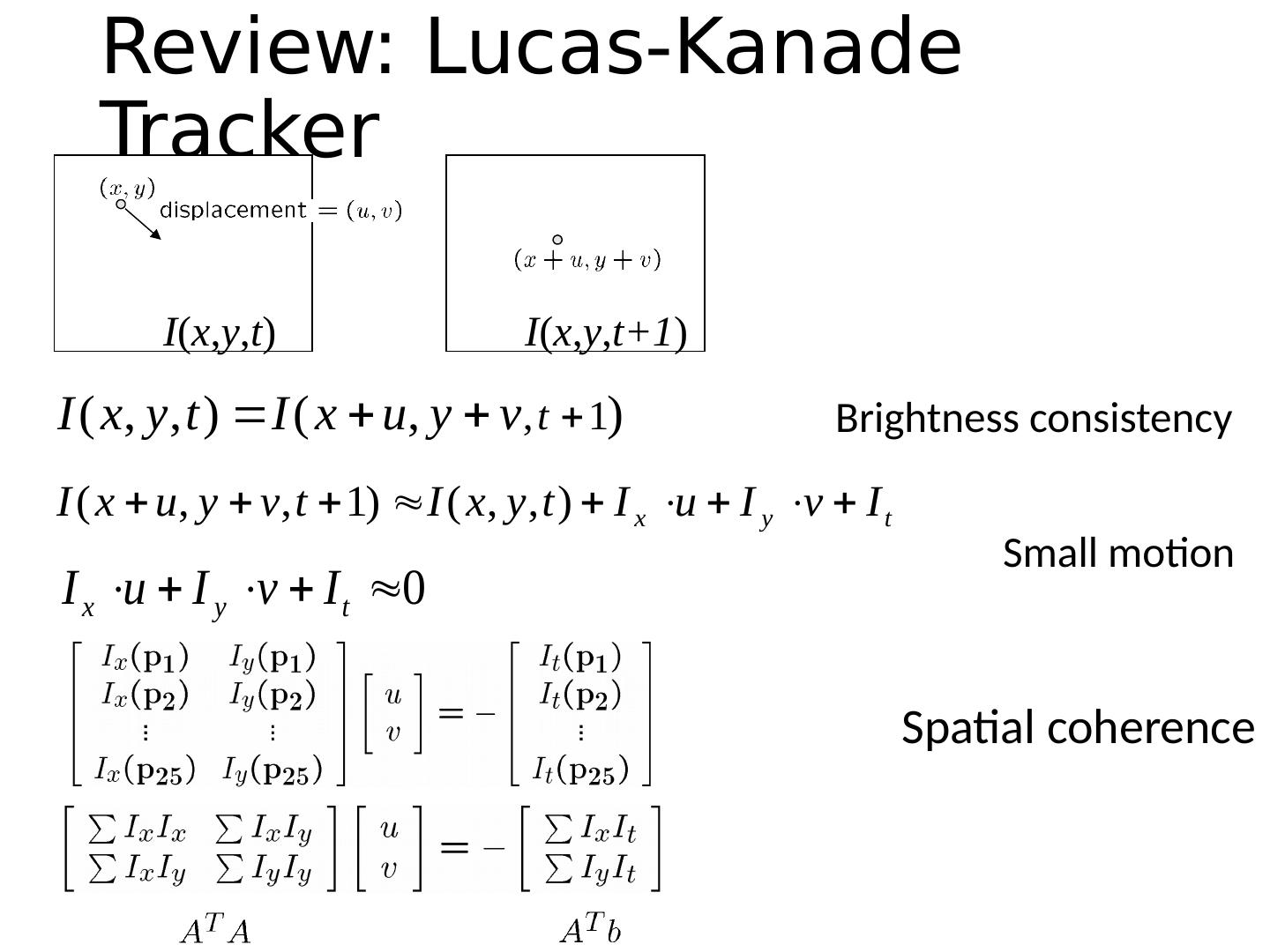
7 .Review: Lucas- Kanade Tracker Brightness consistency I ( x , y , t ) I ( x , y , t+1 ) Small motion Spatial coherence

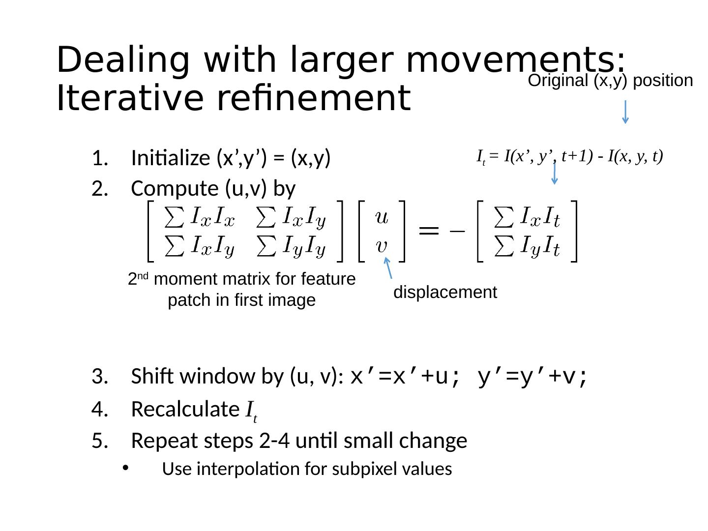
8 .Dealing with larger movements: Iterative refinement Initialize (x’,y’) = (x,y) Compute (u,v) by Shift window by (u, v): x’ = x’+u ; y’= y’+v ; Recalculate I t Repeat steps 2-4 until small change Use interpolation for subpixel values 2 nd moment matrix for feature patch in first image displacement I t = I(x’, y’, t+1) - I(x, y, t) Original (x,y) position

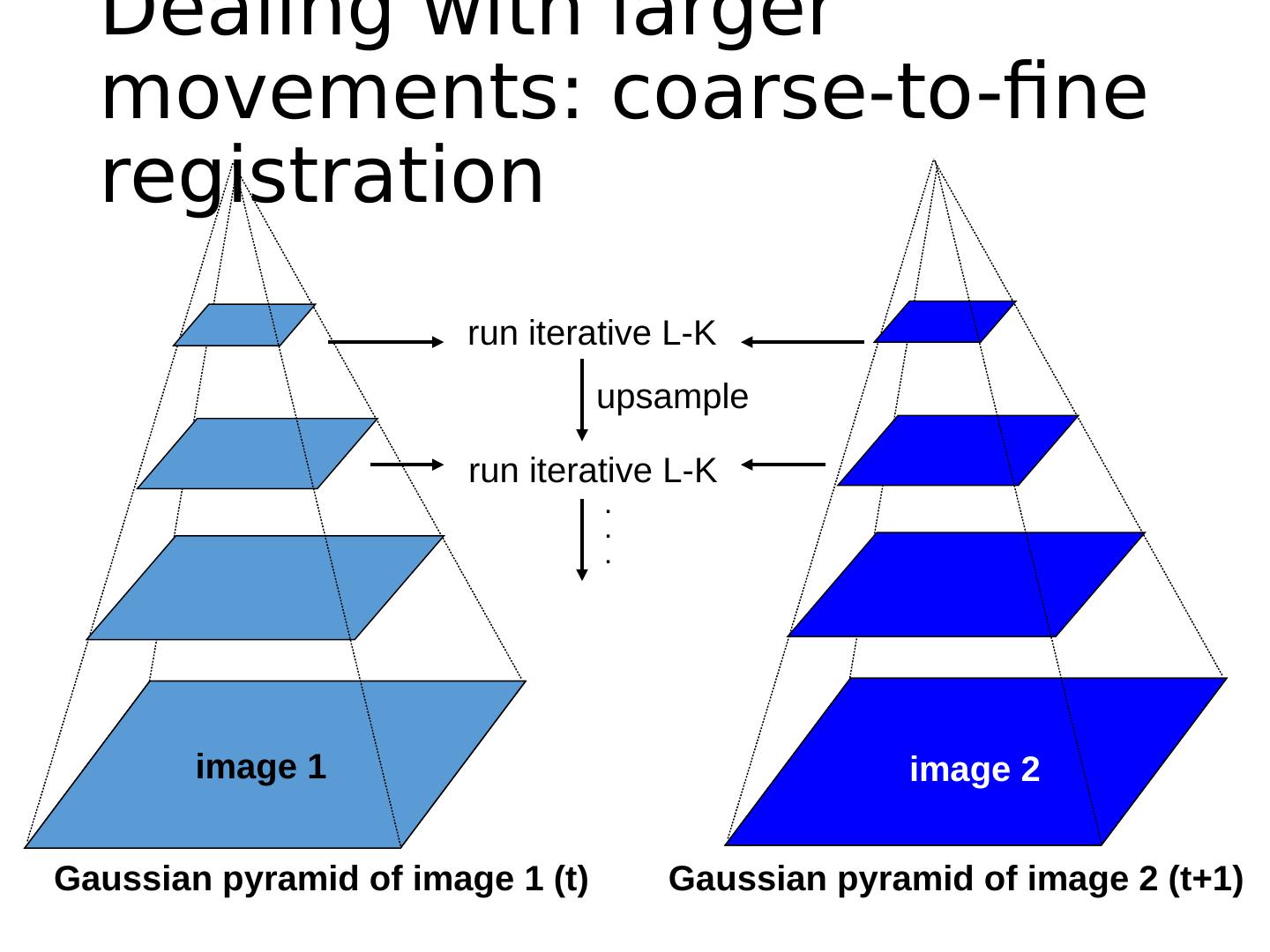
9 .image I image J Gaussian pyramid of image 1 (t) Gaussian pyramid of image 2 (t+1) image 2 image 1 Dealing with larger movements: coarse-to-fine registration run iterative L-K run iterative L-K upsample . . .

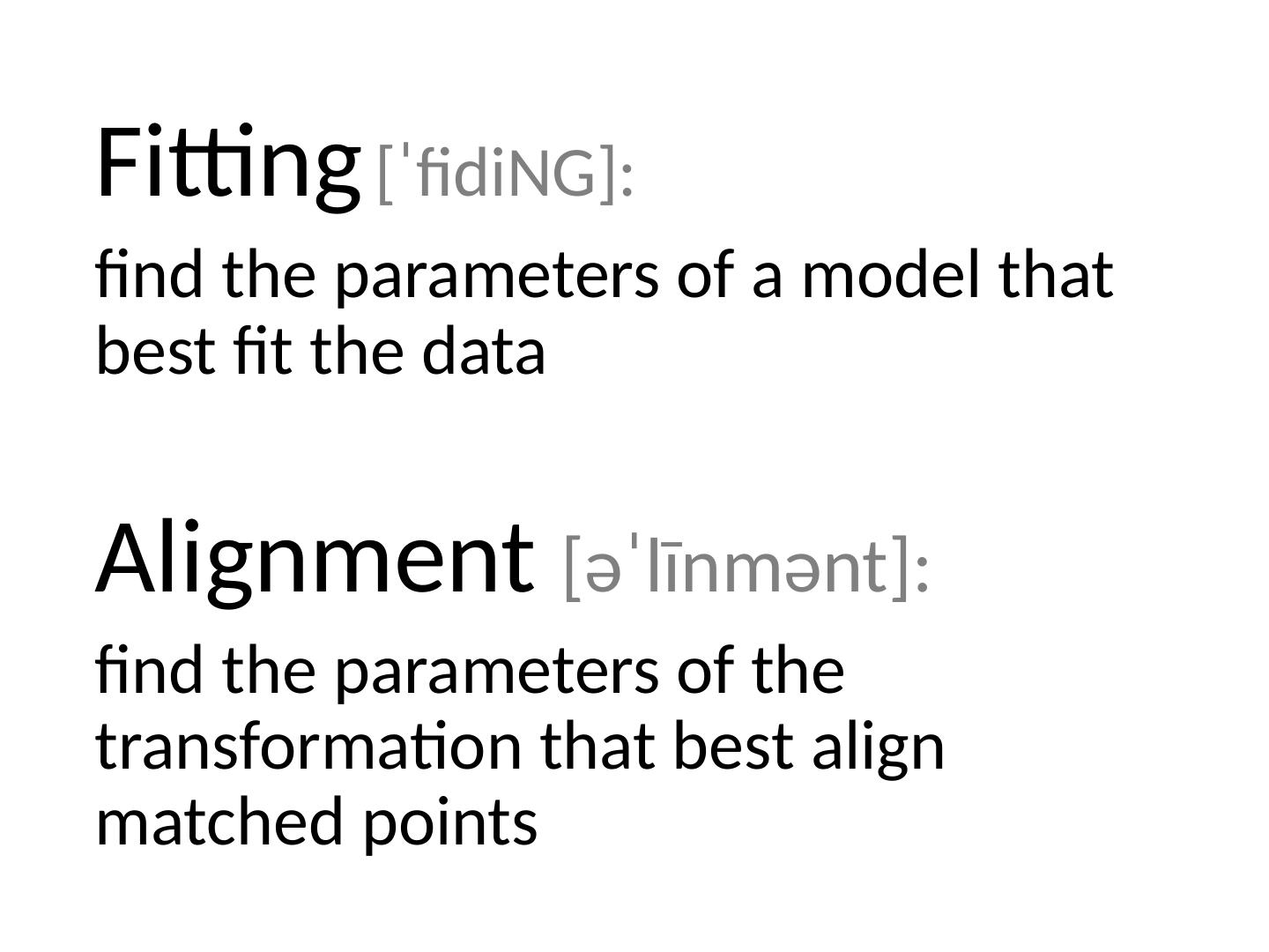
10 .Fitting [ ˈ fidiNG ]: find the parameters of a model that best fit the data Alignment [ əˈlīnmənt ]: find the parameters of the transformation that best align matched points

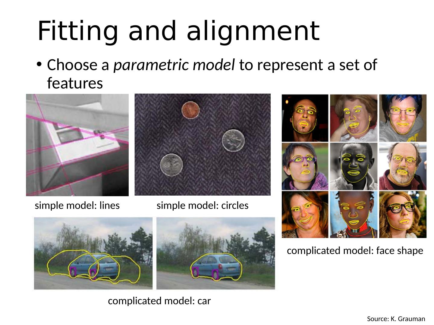
11 .Source: K. Grauman Fitting and alignment Choose a parametric model to represent a set of features simple model: lines simple model: circles complicated model: car complicated model: face shape

12 .Fitting and Alignment -Design challenges Design a suitable goodness of fit measure Similarity should reflect application goals Encode robustness to outliers and noise Design an optimization method Avoid local optima Find best parameters quickly

13 .Fitting and Alignment: Methods Global optimization / Search for parameters Least squares fit Robust least squares Iterative closest point (ICP) Hypothesize and test Generalized Hough transform RANSAC

14 .Simple example: Fitting a line

15 .Least squares line fitting Data: ( x 1 , y 1 ), …, ( x n , y n ) Line equation: y i = m x i + b Find ( m , b ) to minimize ( x i , y i ) y=mx+b Matlab : p = A \ y; Modified from S. Lazebnik

16 .Problem with “vertical” least squares Not rotation-invariant Fails completely for vertical lines Slide from S. Lazebnik

17 .Total least squares If ( a 2 +b 2 = 1) then Distance between point ( x i , y i ) and line ax+by+c =0 is | ax i + by i + c | ( x i , y i ) ax+by+c =0 Unit normal: N= ( a, b ) Slide modified from S. Lazebnik proof: http://mathworld.wolfram.com/Point-LineDistance2-Dimensional.html

18 .Total least squares If ( a 2 +b 2 = 1) then Distance between point ( x i , y i ) and line ax+by+c =0 is | ax i + by i + c | Find ( a , b , c) to minimize the sum of squared perpendicular distances ( x i , y i ) ax+by+c =0 Unit normal: N= ( a, b ) Slide modified from S. Lazebnik

19 .Total least squares Find ( a , b , c ) to minimize the sum of squared perpendicular distances ( x i , y i ) ax+by+c =0 Unit normal: N= ( a, b ) Solution is eigenvector corresponding to smallest eigenvalue of A T A See details on Raleigh Quotient: http://en.wikipedia.org/wiki/Rayleigh_quotient Slide modified from S. Lazebnik

20 .Recap: Two Common Optimization Problems Problem statement Solution Problem statement Solution ( matlab )

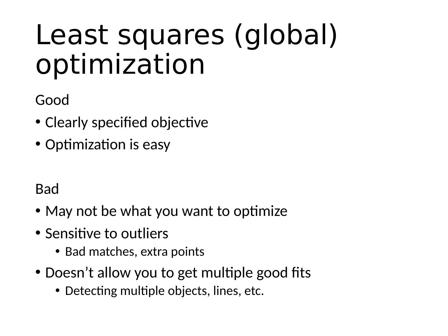
21 .Least squares (global) optimization Good Clearly specified objective Optimization is easy Bad May not be what you want to optimize Sensitive to outliers Bad matches, extra points Doesn’t allow you to get multiple good fits Detecting multiple objects, lines, etc.

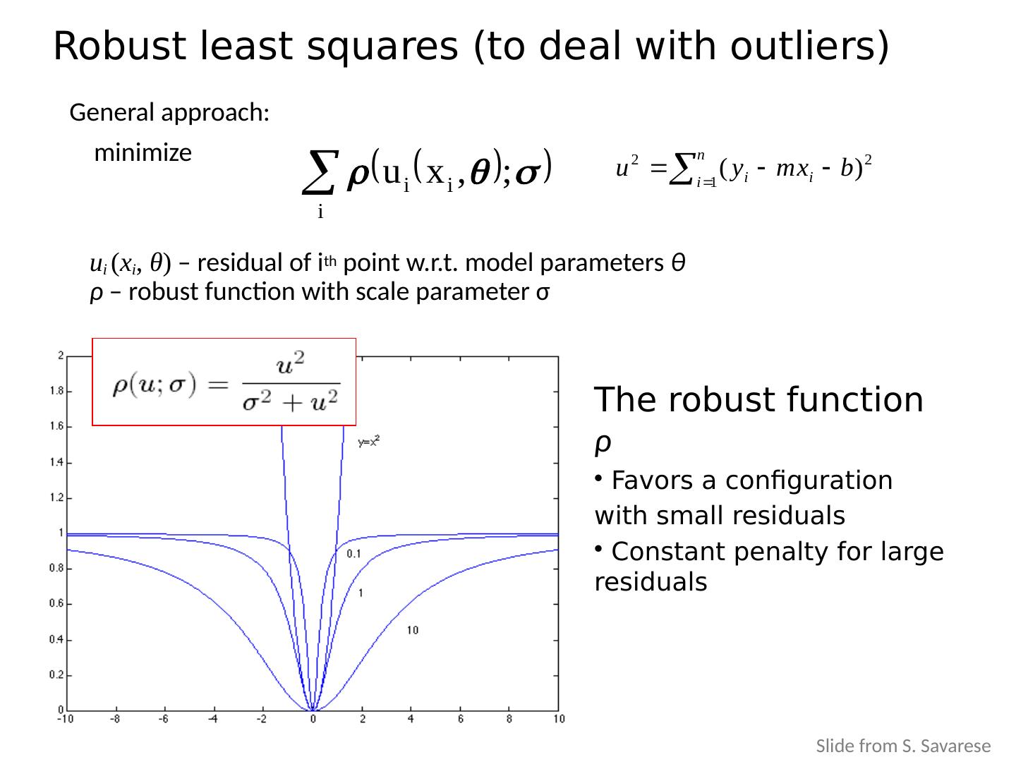
22 .Robust least squares (to deal with outliers) General approach: minimize u i ( x i , θ ) – residual of i th point w.r.t . model parameters θ ρ – robust function with scale parameter σ The robust function ρ Favors a configuration with small residuals Constant penalty for large residuals Slide from S. Savarese

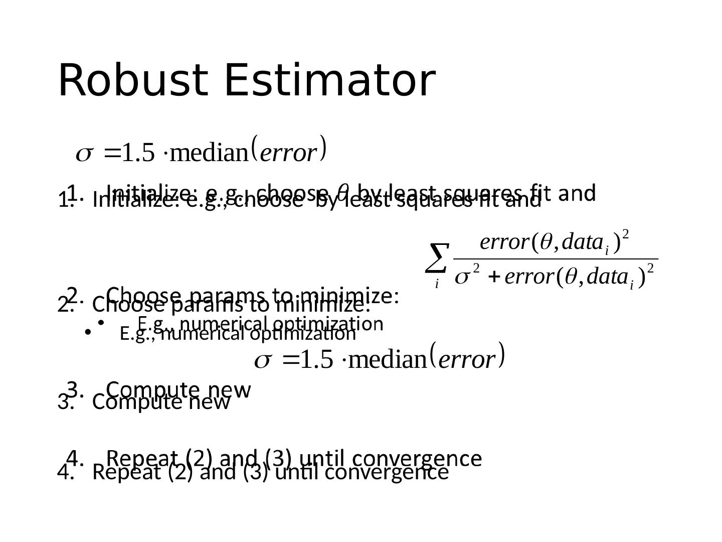
23 .Robust Estimator Initialize: e.g., choose by least squares fit and Choose params to minimize: E.g., numerical optimization Compute new Repeat (2) and (3) until convergence  

24 .Other ways to search for parameters (for when no closed form solution exists) Line search F or each parameter, step through values and choose value that gives best fit Repeat (1) until no parameter changes Grid search Propose several sets of parameters, evenly sampled in the joint set Choose best (or top few) and sample joint parameters around the current best; repeat Gradient descent Provide initial position (e.g., random) Locally search for better parameters by following gradient

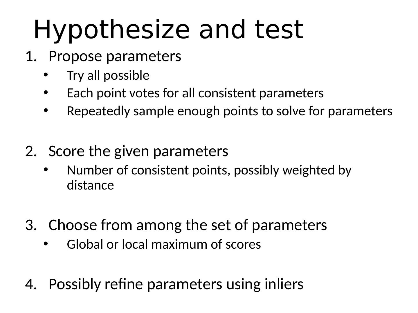
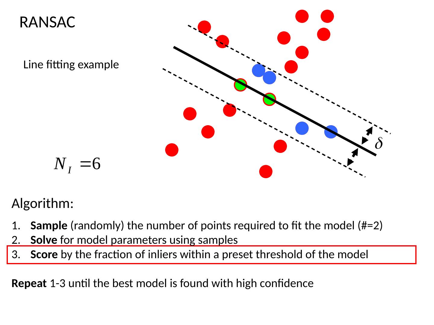
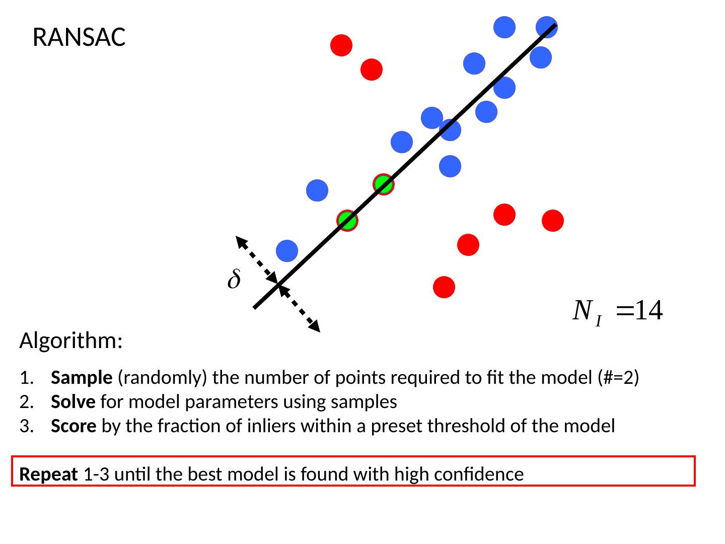
25 .Hypothesize and test Propose parameters Try all possible Each point votes for all consistent parameters Repeatedly sample enough points to solve for parameters Score the given parameters Number of consistent points, possibly weighted by distance Choose from among the set of parameters Global or local maximum of scores Possibly refine parameters using inliers

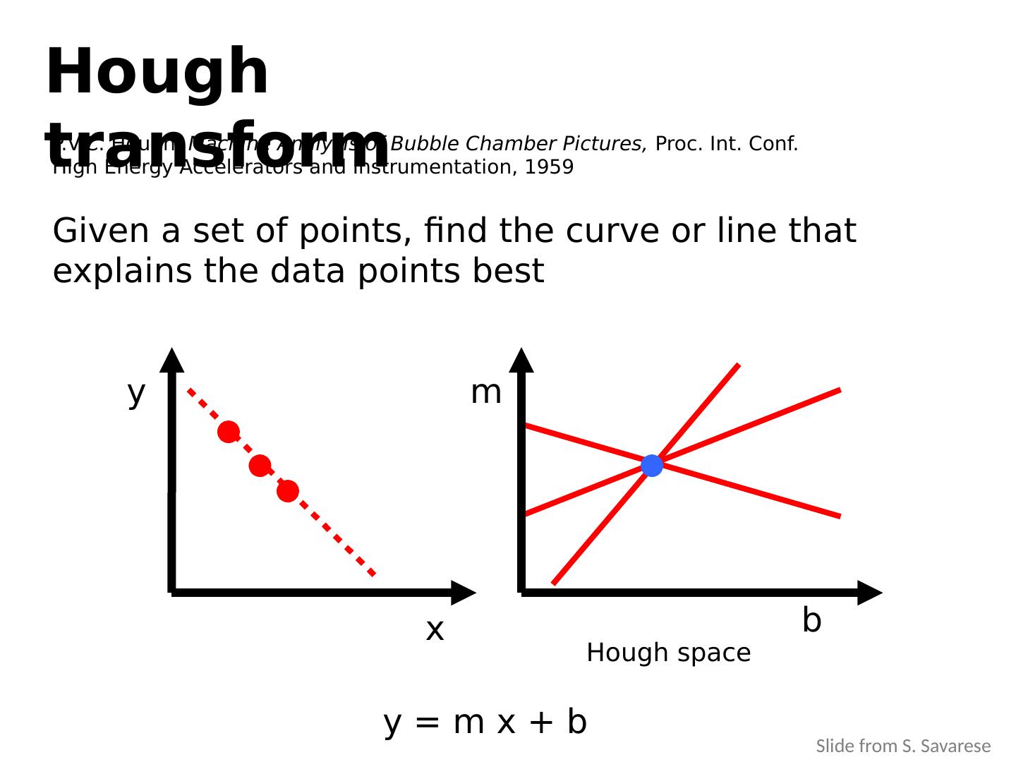
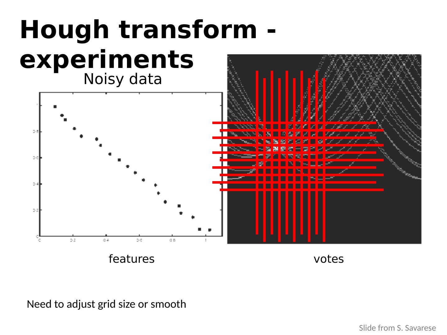
26 .Hough Transform: Outline Create a grid of parameter values Each point votes for a set of parameters, incrementing those values in grid Find maximum or local maxima in grid

27 .x y b m y = m x + b Hough transform Given a set of points, find the curve or line that explains the data points best P.V.C. Hough, Machine Analysis of Bubble Chamber Pictures, Proc. Int. Conf. High Energy Accelerators and Instrumentation, 1959 Hough space Slide from S. Savarese

28 .x y b m x y m 3 5 3 3 2 2 3 7 11 10 4 3 2 3 1 4 5 2 2 1 0 1 3 3 b Hough transform Slide from S. Savarese

29 .x y Hough transform Issue : parameter space [ m,b ] is unbounded… P.V.C. Hough, Machine Analysis of Bubble Chamber Pictures, Proc. Int. Conf. High Energy Accelerators and Instrumentation, 1959 Hough space Use a polar representation for the parameter space Slide from S. Savarese