基于Spark的深度神经网络超参数选择与自适应模型整定

1 .Hyper-Parameter Selection and Adaptive Model Tuning for Deep Neural Networks YongGang Hu, Chao Xue, IBM #AssignedHashtagGoesHere 

2 . Outline • Hyper-parameter selections & Neural network search – Bayesian optimization – Hyperband – Reinforcement learning • Transfer AutoML – Using historical hyper-parameter configurations for different tasks – Joint optimization with AutoML and finetune • Training visualization and Interactive tuning • Real world experience and Implementation 2 

3 . From Hyper parameter/Network Search to On-line Tuning Image Hyper-parameter & Network Real-time monitor for running application recognition Search learning curve weight/gradient/a ctivation Deep Learning Applications optimizing criterion and histogram and Object procedure model Monitor detection norm parameters parameters example: learning example: number of worst cases of rate, batch size, hidden units, number training samples momentum, learning of layers, filter kernel Optimize rate scheme size, max-pool size, weight decay Real-time adviser for running application Translation overflow check the training Advice underfitting process Others overfitting divergence convergence 

4 .Standard AutoML--from Random search, Bayesian Optimization to Reinforcement Learning Hyperparameters auto Neural Network auto selected selected Adaptive Random Search u1 uM (Hyperband) s1 Q Bayesian Reinforceme Optimization nt Learning sN 4 

5 . Results of AdaRandom and Bayesian Optimization for Object detection • The raw data (no data augment) mAP § The average results for the three (HPP) Machine IBM P8 hyperparameters combinations at 4000 0.8 iterations are (0.49, 0.52, 0.55), that is, GPU Tesla K80 using AdaRandom and Bayesian 0.6 optimization recommended HPP, you can GPU MEM 10G gain 6% and 12% in the average results 0.4 comparing to default setting. AdaRandom 0.2 method has more variance among CPU ppc64le different tries(train-test dataset split). The 0 Bayesian models are more stable while CPU cores 160 avg Best case Worst case having better average performance. § The below pictures show accuracy during MEM 55G default the 0-4000 iterations, with different tries, AdaRandom(HyperBand) under the two HPP configurations. We Frequency 3.5 GHz can see that: 1) It can be early stopped at Bayesian Optimization about 1300 iterations. 2) the performance OS Ubuntu with different tries differ significantly, it 14.04 caused by in some tries, training dataset caffe version Py-faster- has the invariance property according to test dataset, but some doesn’t have. It rcnn need to augment data to gain the stable Dataset User-defined performance. 3) different HPP combinations(models) may have different Model vgg16 sensitivity to the different tries. 5 

6 . Evaluations with Acoustic Applications • We implement the AdaRandom (adaptive random search scheme) and Reinforce (reinforcement learning search scheme) methods to generate deep learning neural network automatically. • We are trying the new methods in different areas. Here is the example for acoustic. Default is the best scheme by manual tuning. Lower complexity Better accuracy More stable Neural Network: C: Convolution, P: pooling, FC: Full connection. Default manual: (9 layers) C(3,32)+C(3,32)+P(3,3)+C(3,64)+C(3,64)+P (3,3)+FC(64)+FC(32)+FC(6) AdaRandom generated: (6 layers) C(3,128)+C(4,64)+C(3,32)+P(3,3)+FC(16)+ FC(6) Reinforce generated: (5 layers) C(3,32)+P(2,2)+P(3,2)+C(5,32)+FC(6) • The best results for the three networks are (0.703,0.673, 0.695) (the smaller the better), that is, using AdaRandom and Reinforce recommended models, you can gain 4.3% and 1.1% in the best results comparisons. The average result of the three networks is (0.817,0.776, 0.763), that is, the DL Insight recommended modes can increase about 5.0% and 6.6% in the average case performance. And from the standard deviation view, the recommended models are clearly more stable. • The CDF (cumulative distribution function) curve is more intuitive to illustrate the comparison of the three models(the more left the better). For example, using reinforce recommended model, ER has more than 60% probability (frequency) less than 0.75, while the default only has the 30%. 6 

7 . Transfer AutoML Architecture Weights and bias Parameter Traditional fine-tune Neural network Hyper-parameter Model Standalone AutoML Collaborative AutoML Dataset group Virtual Dataset Dog Car Unknown Dataset 7 

8 . AutoML process Server Clients White-box Server analysis RL Parallelization B Upload Knowledge base datasets Spark Clients Benchmark HyperBand Black-box models analysis selection Path 1 Virtual datasets group Bayesian Path 1 Joint Optimization Model with transfer selection learning 

9 . Challenges for AutoML with Transfer Learning • Training small user dataset leads to convergence problem à Transfer learning is needed • When considering transfer learning, the pretrained model need to be chosen, usually in the computer vision, we choose image-net as the base dataset to get the initial weights as the pretrained model, but it can’t fit many specific user datasets. • To solve this transfer learning’s problem, we can let the user to classify his dataset into some predefined categories, and in each category, the pretrained model was trained separately. It can improve the performance of transfer learning but involve user’s intervention with their datasets. • Using AutoML with transfer learning can improve transfer learning’s performance without user’s intervention. But considering the transfer learning’s properties, there are two challenges for AutoML: – Since reusing the initial weights, transfer learning limits the searching space of AutoML, how to use AutoML based on the pretrained model is a question. – We can’t use AutoML to build one model for every user dataset, it is too expensive. How to reuse the model for transfer learning is a question. 9 

10 .Joint optimization: AutoML with the fine-tune 

11 .Search space: 1) Neural network at the last stage: layer { name: "last_fc" Example: type: "InnerProduct" layer { c p c p fc param { bottom: "pool1" top: "last_fc" lr_mult: LR_MULT_C_W_0 param { 2) Below hyper-parameter decay_mult: DECAY_MULT_C_W_0 lr_mult: LR_MULT_FC_W_0 } decay_mult: param { DECAY_MULT_FC_W_0 lr_mult: LR_MULT_C_B_0 } • lr_policy: LR_POLICY layer { decay_mult: param { stepsize: STEPSIZE name: "conv0_relu" DECAY_MULT_C_B_0 type: TYPE_C_AF_0 lr_mult: LR_MULT_FC_B_0 gamma: GAMMA } bottom: "conv0" decay_mult: momentum: MOMENTUM convolution_param { top: "conv0" num_output: NUM_OUTPUT_0 DECAY_MULT_FC_B_0 solver_mode: GPU } } pad: PAD_0 max_iter: MAX_ITER inner_product_param { layer { kernel_size: KERNEL_SIZE_C_0 test_iter: TEST_ITER name: "pool1" num_output: OUTPUT_NUMS group: GROUP_0 test_interval: TEST_INTERVAL type: "Pooling" weight_filler { weight_filler { base_lr: BASE_LR bottom: "conv0" type: TYPE_C_W_0 type: TYPE_FC_W_0 weight_decay: WEIGHT_DECAY top: "pool1" std: STD_C_W_0 std: STD_FC_W_0 solver_type: SGD pooling_param { } } pool: AVE bias_filler { bias_filler { kernel_size: type: TYPE_C_B_0 KERNEL_SIZE_P_0 type: TYPE_FC_B_0 std: STD_C_B_0 stride: STRIDE_P_0 std: STD_FC_B_0 } } } } } } } } 

12 .Results and Analysis Accuracy 1.2 1 Advantages of AutoML with finetune: 0.8 (+) Best accuracy (+) Most stable 0.6 (+) Don’t need separate 0.4 pretrained models by predefining dataset 0.2 categories. No user’s interventions. 0 Food(30 epoch) TV show(10 Car(50 epoch) Sence(100 Action(20 epoch) epoch) epoch) GoogleCAM+Finetune(Imagenet) GoogleCAM+Finetune(imagenet+ same category dataset) AutoML+Finetune(Imagenet) 

13 .Training Monitoring & Interactive Tuning of Hyper Parameters Expert optimization advice for hyper parameter selection and tuning Traffic light alerting for required parameter optimization with early stop advice and more CPU, GPU, memory utilization info, comms overhead, +++ 13 

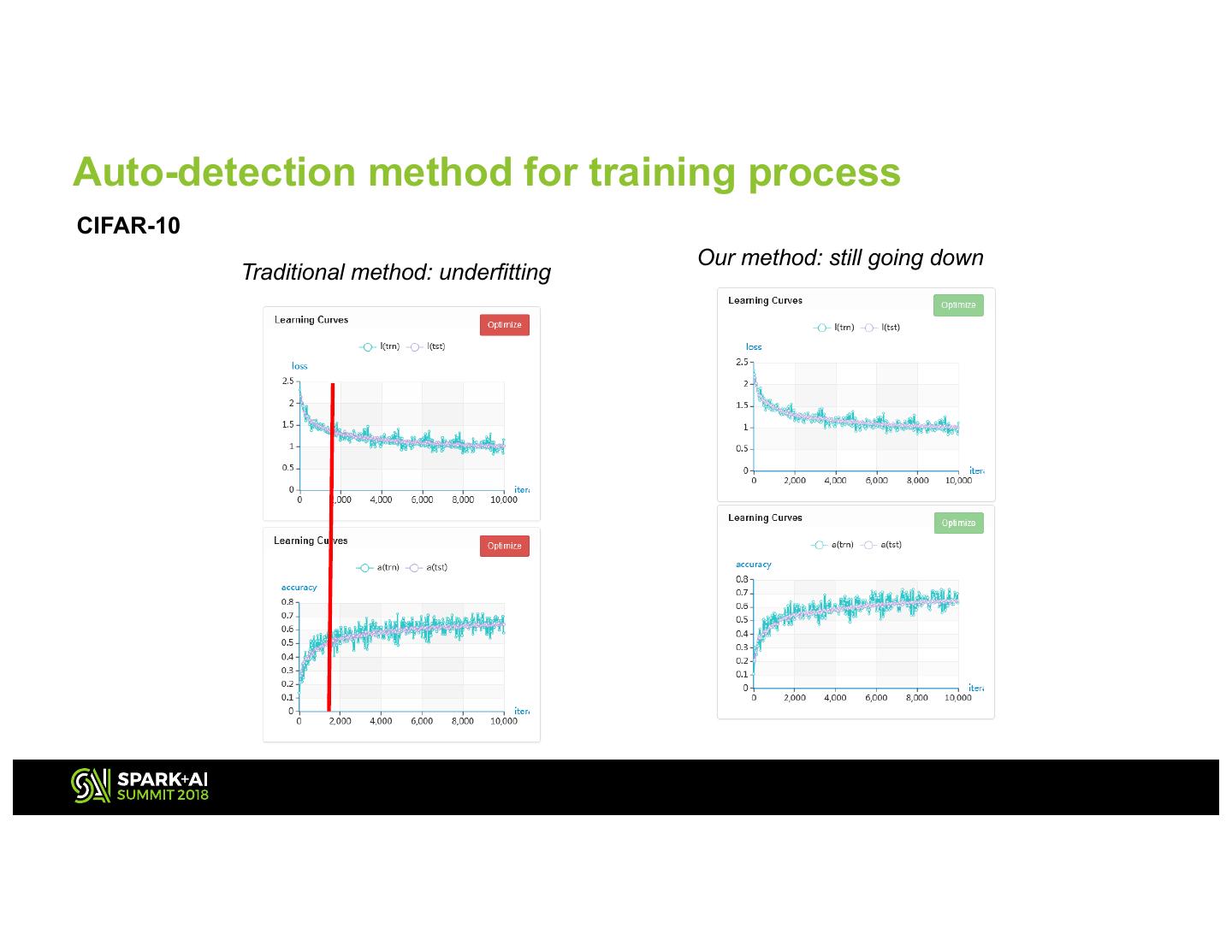
14 . Auto-detection method for training process CIFAR-10 Our method: still going down Traditional method: underfitting 14 

15 . Auto-detection method for training process MNIST Traditional method: underfitting Our method: good game 15 

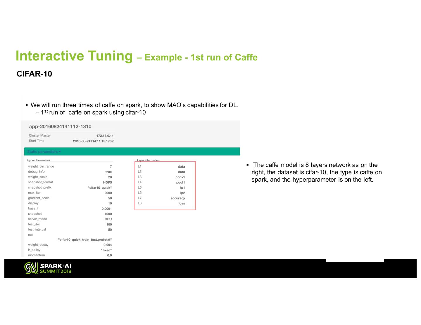
16 .Interactive Tuning – Example - 1st run of Caffe CIFAR-10 16 

17 .Interactive Tuning – Example - 1st run of Caffe 17 

18 .Interactive Tuning – Example - 2nd run of Caffe 18 

19 .Interactive Tuning – Example - 2nd run of Caffe 19 

20 .Interactive Tuning – Example -3rd run of Caffe 20 

21 .Interactive Tuning – Example - 3rd run of Caffe 21 

22 . Interactive Tuning - Example: “Applause” datasets Hyperparameters in suggestions Parameters batch mAP at early runs AP mAP base_lr weight_decay momentum early stop size/rpn split ratio max_iters display stop iteration batch size yes iter=370 applause01 0.001 0.0005 0.9 128/256 0.7(94/39) 2000 10 appl = 0.3409 0.3409 m AP=0.221060 divergence Good judgement 2 

23 . Learning Curve Trend Judgement – ‘Applause’ (Continue) Hyperparameters in suggestions Parameters batch mAP at early runs weight_de momentu AP mAP base_lr early stop size/rpn split ratio max_iters display stop iteration cay m batch size yes iter=350 applause-aug01-01 0.001 0.0005 0.9 128/256 0.7(98/42) 2000 10 AP for appl = 0.4848 0.4848 m AP=0.313152 divergence Good judgement 2 

24 . Learning Curve Trend Judgement – ‘Applause’ (Continue) Hyperparameters in suggestions Parameters batch mAP at early runs weight_de momentu AP mAP base_lr early stop size/rpn split ratio max_iters display stop iteration cay m batch size iter=1510 applause-aug03-01 0.001 0.0005 0.9 128/256 0.7(164/69) 2000 10 AP for appl = 0.7847 0.7847 m AP=0.784068 Good judgement 2 

25 .Hyper-Parameter Search Implementation Search hyper-parameters space : – Learning rate – Decay rate – Batch size – Optimizer: • GradientDecedent, • Adadelta, • … – Momentum (for some optimizers) – LSTM hidden unit size Random, Bayesian, TPE Based Search Types IBM CONFIDENTIAL 25 

26 .Hyper-Parameter Search Implementation TPE Random Tree-based Parzen Estimator Bayesian Spark search jobs are generated dynamically and executed in parallel Multitenant Spark Cluster IBM Spectrum Conductor Think 2018 / 5613A.pdf / March 22, 2018 / © 2018 IBM Corporation 26 

27 .Hyper-Parameter Search Implementation HPTAlgorithm TuneInputParam inputP ModelTuningMgrl TuningJobCtr jobctl startModelAutoTuning() search() stopModelAutoTuning() deleteModelAutoTuning() BayesianAlg PythonAlg TuningTask RandomAlg UserPlugInAl (Thread) g run() TPEAlg TuningFrameworkMgr initialize() TuningJobCtr getLossValueFromLog() runTuningJobs() prepareJob() PytorchFrameworkMg CoSFrameWorkMgrl rl SparkTuningJobCtrI TuningFrameworkMgr frameworkMgr TfFrameworkMgrl 

28 .Enterprise Class Deep Learning Solution IBM Spectrum Conductor Deep Learning Impact, IBM PowerAI, IBM Storage Tensorflow Caffe Workload Management / Scheduling Monitoring & Reporting Native Services Management Deep Resource Management & Orchestration Learning Impact Services & Support IBM PowerAI Red Hat Linux IBM Power Systems … x86 IBM Storage IBM CONFIDENTIAL 28 

29 . Reference • [1] David Schaffer, Darrell Whitley and Larry J Eshelman, Combinations of genetic algorithms and neural networks: A survey of the state of the art. International Workshop on Combinations of Genetic Algorithms and Neural Networks, 1992. • [2] J.Snoek, H.Larochelle and R.P.Adams, Practical Bayesian optimization of machine learning algorithms. In Advances in Neural Information Processing Systems(NIPS), 2012. 
 • [3] Bergstra, James and Yoshua Bengio, Random search for hyper-parameter optimization. Journal of Machine Learning Research, 2012. 
 • [4] Lisha Li, Kevin Jamieson and Giulia DeSalvo, HYPERBAND: BANDIT- BASED CONFIGURATION EVALUATION FOR HYPERPARAMETER OPTIMIZATION. ICLR, 2017. 
 • [5] James Bergstra, etc. Algorithms for Hyper-Parameter Optimization. Proceedings of the IEEE, 2012. 
 • [6] Bowen Baker, Otkrist Gupta, Nikhil Naik and RameshRaskar, DESIGNING NEURAL NETWORK ARCHITECTURES USING REINFORCEMENT LEARNING. ICLR, 2017.