The Data Engineers Guide to Apache Spark

1 .The Data Engineer’s Guide to 

2 .Preface Apache Spark has seen immense growth over the past several years. The size and scale of Spark Summit 2017 is a true reflection of innovation after innovation that has made itself into the Apache Spark project. Databricks is proud to share excerpts from the upcoming book, Spark: The Definitive Guide. Enjoy this free preview copy, courtesy of Databricks, of chapters 2, 3, 4, and 5 and subscribe to the Databricks blog for upcoming chapter releases. 2 

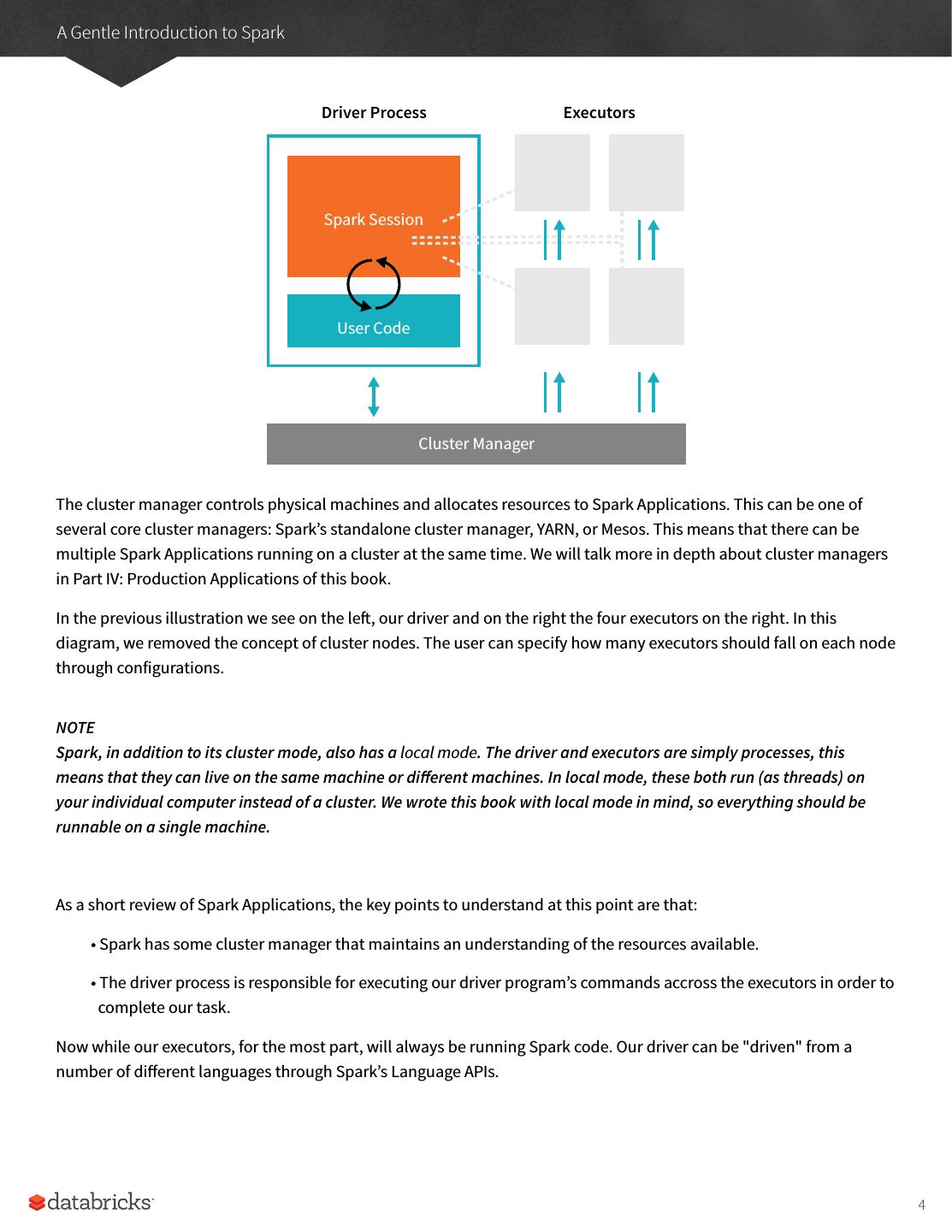
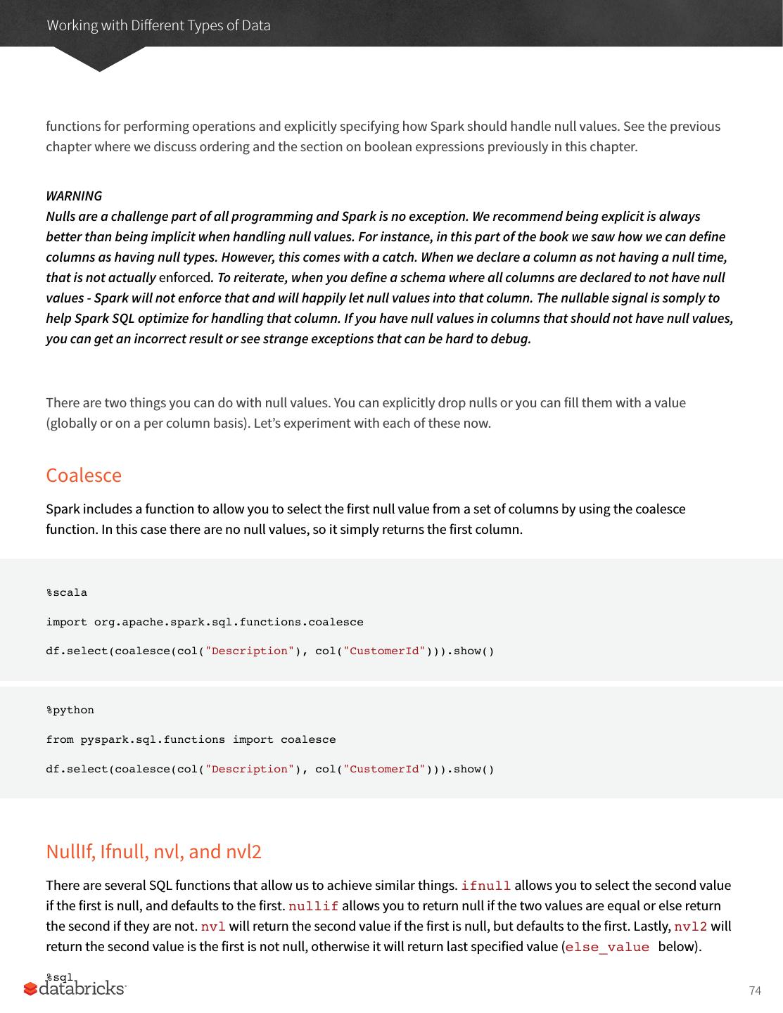
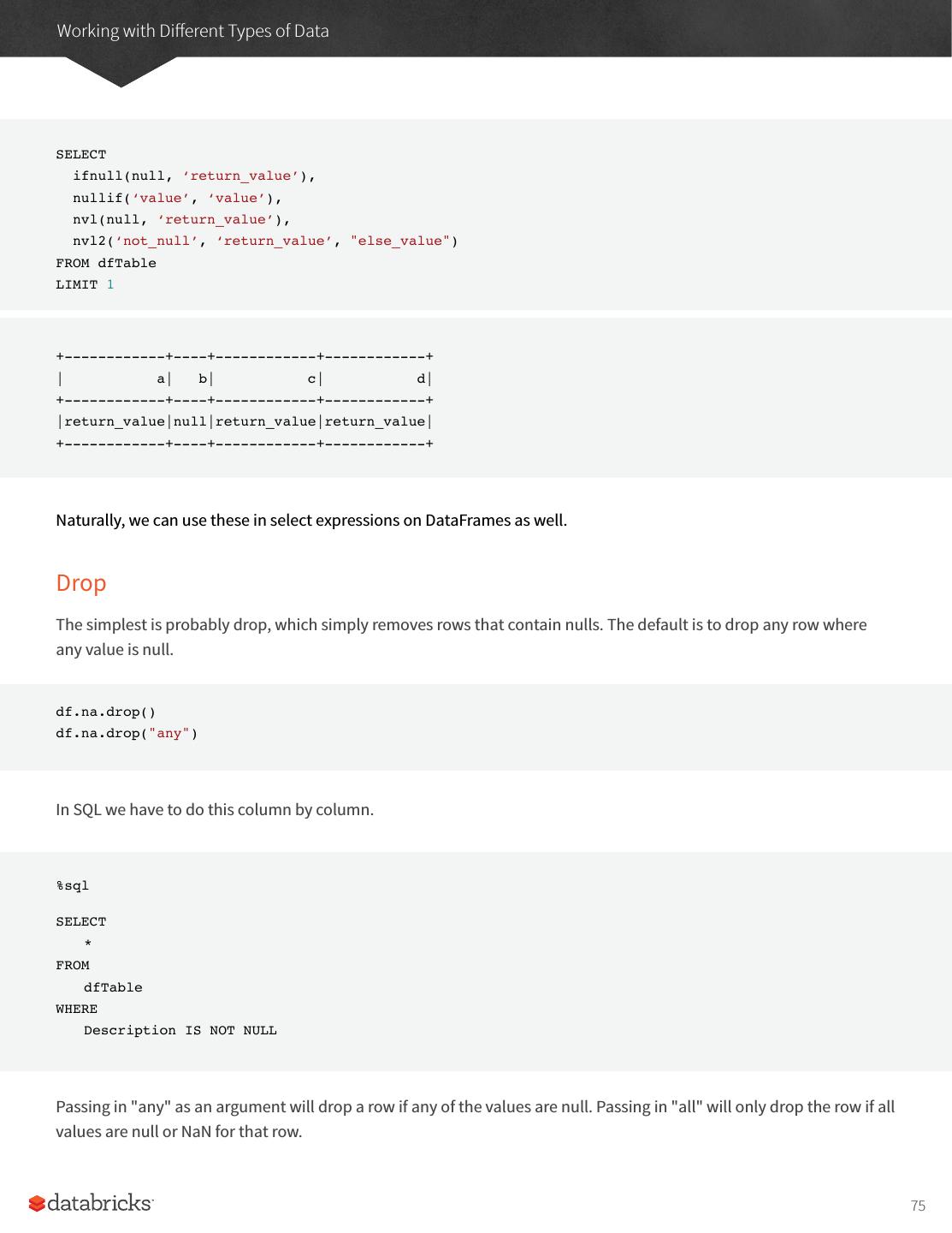
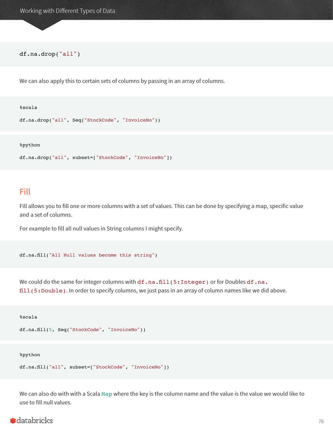
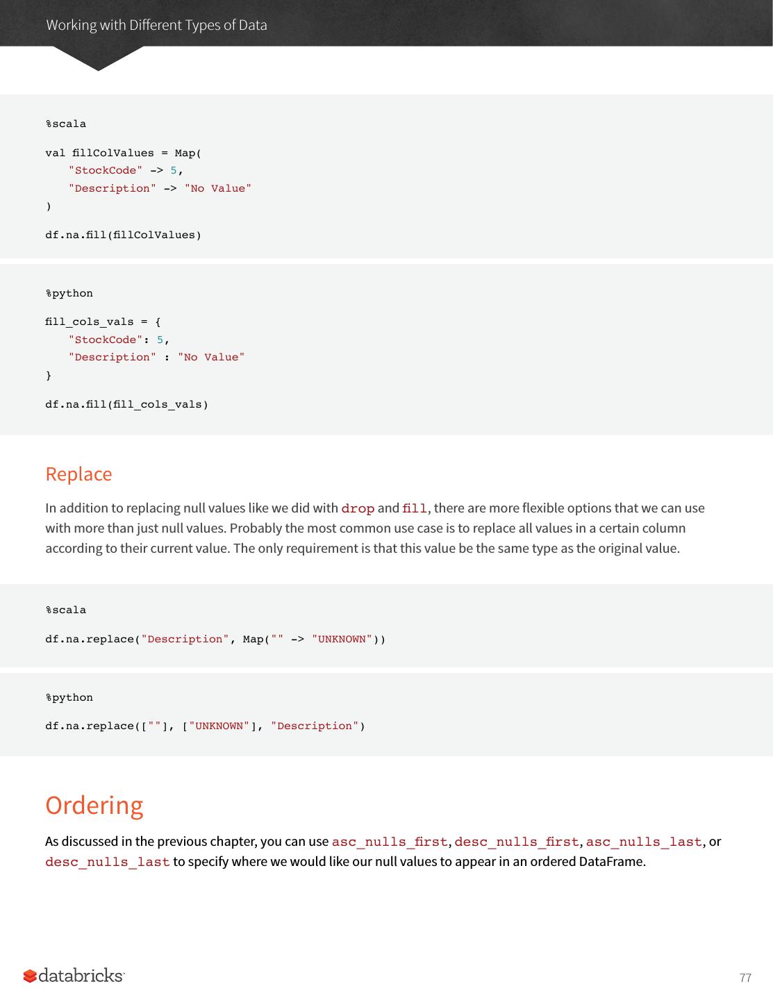
3 .A Gentle Introduction to Spark Now that we took our history lesson on Apache Spark, it’s time to start using it and applying it! This chapter will present a gentle introduction to Spark - we will walk through the core architecture of a cluster, Spark Application, and Spark’s Structured APIs using DataFrames and SQL. Along the way we will touch on Spark’s core terminology and concepts so that you are empowered start using Spark right away. Let’s get started with some basic background terminology and concepts. Spark’s Basic Architecture Typically when you think of a "computer" you think about one machine sitting on your desk at home or at work. This machine works perfectly well for watching movies or working with spreadsheet software. However, as many users likely experience at some point, there are some things that your computer is not powerful enough to perform. One particularly challenging area is data processing. Single machines do not have enough power and resources to perform computations on huge amounts of information (or the user may not have time to wait for the computation to finish). A cluster, or group of machines, pools the resources of many machines together allowing us to use all the cumulative resources as if they were one. Now a group of machines alone is not powerful, you need a framework to coordinate work across them. Spark is a tool for just that, managing and coordinating the execution of tasks on data across a cluster of computers. The cluster of machines that Spark will leverage to execute tasks will be managed by a cluster manager like Spark’s Standalone cluster manager, YARN, or Mesos. We then submit Spark Applications to these cluster managers which will grant resources to our application so that we can complete our work. Spark Applications Spark Applications consist of a driver process and a set of executor processes. The driver process runs your main() function, sits on a node in the cluster, and is responsible for three things: maintaining information about the Spark Application; responding to a user’s program or input; and analyzing, distributing, and scheduling work across the executors (defined momentarily). The driver process is absolutely essential - it’s the heart of a Spark Application and maintains all relevant information during the lifetime of the application. The executors are responsible for actually executing the work that the driver assigns them. This means, each executor is responsible for only two things: executing code assigned to it by the driver and reporting the state of the computation, on that executor, back to the driver node. 3 

4 .A Gentle Introduction to Spark Driver Process Executors Spark Session User Code Cluster Manager The cluster manager controls physical machines and allocates resources to Spark Applications. This can be one of several core cluster managers: Spark’s standalone cluster manager, YARN, or Mesos. This means that there can be multiple Spark Applications running on a cluster at the same time. We will talk more in depth about cluster managers in Part IV: Production Applications of this book. In the previous illustration we see on the left, our driver and on the right the four executors on the right. In this diagram, we removed the concept of cluster nodes. The user can specify how many executors should fall on each node through configurations. NOTE Spark, in addition to its cluster mode, also has a local mode. The driver and executors are simply processes, this means that they can live on the same machine or different machines. In local mode, these both run (as threads) on your individual computer instead of a cluster. We wrote this book with local mode in mind, so everything should be runnable on a single machine. As a short review of Spark Applications, the key points to understand at this point are that: • Spark has some cluster manager that maintains an understanding of the resources available. • The driver process is responsible for executing our driver program’s commands accross the executors in order to complete our task. Now while our executors, for the most part, will always be running Spark code. Our driver can be "driven" from a number of different languages through Spark’s Language APIs. 4 

5 .A Gentle Introduction to Spark Spark’s Language APIs Spark’s language APIs allow you to run Spark code from other langauges. For the most part, Spark presents some core "concepts" in every language and these concepts are translated into Spark code that runs on the cluster of machines. If you use the Structured APIs (Part II of this book), you can expect all languages to have the same performance characteristics. NOTE This is a bit more nuanced than we are letting on at this point but for now, it’s the right amount of information for new users. In Part II of this book, we’ll dive into the details of how this actually works. Scala Spark is primarily written in Scala, making it Spark’s "default" language. This book will include Scala code examples wherever relevant. Java Even though Spark is written in Scala, Spark’s authors have been careful to ensure that you can write Spark code in Java. This book will focus primarily on Scala but will provide Java examples where relevant. Python Python supports nearly all constructs that Scala supports. This book will include Python code examples whenever we include Scala code examples and a Python API exists. SQL Spark supports ANSI SQL 2003 standard. This makes it easy for analysts and non-programmers to leverage the big data powers of Spark. This book will include SQL code examples wherever relevant R Spark has two commonly used R libraries, one as a part of Spark core (SparkR) and another as a R community driven package (sparklyr). We will cover these two different integrations in Part VII: Ecosystem. 5 

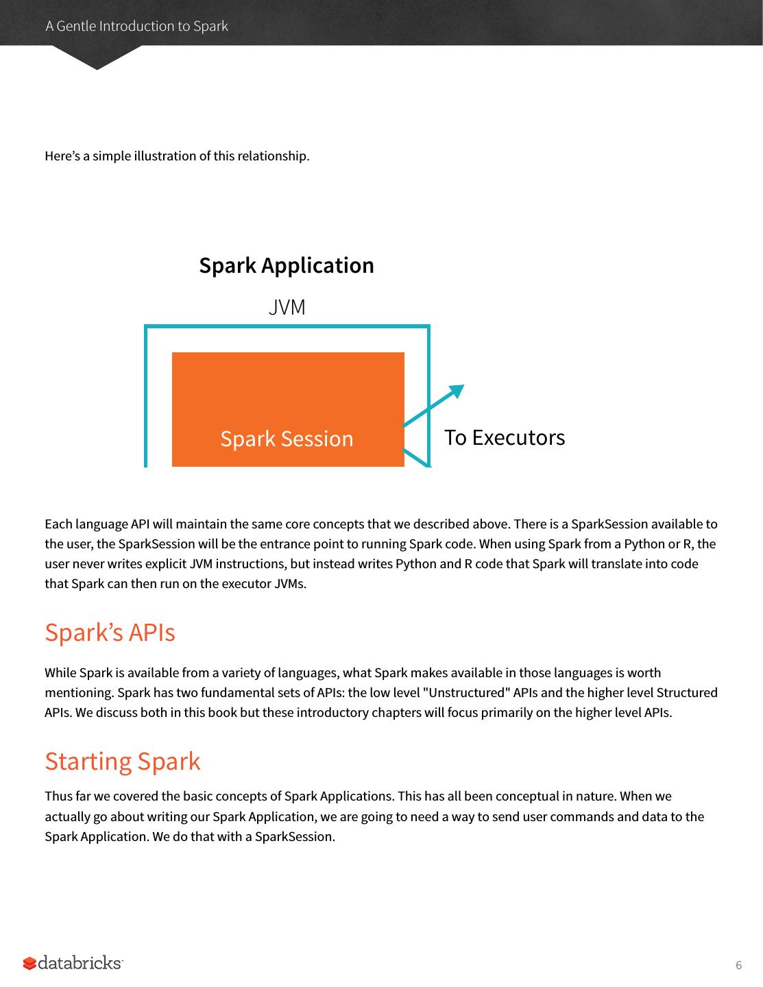
6 .A Gentle Introduction to Spark Here’s a simple illustration of this relationship. Spark Application JVM Spark Session To Executors Each language API will maintain the same core concepts that we described above. There is a SparkSession available to the user, the SparkSession will be the entrance point to running Spark code. When using Spark from a Python or R, the user never writes explicit JVM instructions, but instead writes Python and R code that Spark will translate into code User Code that Spark can then run on the executor JVMs. Spark’s APIs While Spark is available from a variety of languages, what Spark makes available in those languages is worth mentioning. Spark has two fundamental sets of APIs: the low level "Unstructured" APIs and the higher level Structured APIs. We discuss both in this book but these introductory chapters will focus primarily on the higher level APIs. Starting Spark Thus far we covered the basic concepts of Spark Applications. This has all been conceptual in nature. When we actually go about writing our Spark Application, we are going to need a way to send user commands and data to the Spark Application. We do that with a SparkSession. 6 

7 .A Gentle Introduction to Spark NOTE To do this we will start Spark’s local mode, just like we did in the previous chapter. This means running ./bin/ spark-shell to access the Scala console to start an interactive session. You can also start Python console with ./bin/pyspark. This starts an interactive Spark Application. There is also a process for submitting standalone applications to Spark called spark-submit where you can submit a precompiled application to Spark. We’ll show you how to do that in the next chapter. When we start Spark in this interactive mode, we implicitly create a SparkSession which manages the Spark Application. When we start it through a job submission, we must go about creating it or accessing it. The SparkSession As discussed in the beginning of this chapter, we control our Spark Application through a driver process. This driver process manifests itself to the user as an object called the SparkSession. The SparkSession instance is the way Spark executes user-defined manipulations across the cluster. There is a one to one correspondance between a SparkSession and a Spark Application. In Scala and Python the variable is available as spark when you start up the console. Let’s go ahead and look at the SparkSession in both Scala and/or Python. spark In Scala, you should see something like: res0: org.apache.spark.sql.SparkSession = org.apache.spark.sql.SparkSession@27159a24 In Python you’ll see something like: <pyspark.sql.session.SparkSession at 0x7efda4c1ccd0> Let’s now perform the simple task of creating a range of numbers. This range of numbers is just like a named column in a spreadsheet. %scala val myRange = spark.range(1000).toDF("number") %python myRange = spark.range(1000).toDF("number") You just ran your first Spark code! We created a DataFrame with one column containing 1000 rows with values from 0 to 999. This range of number represents a distributed collection. When run on a cluster, each part of this range of numbers exists on a different executor. This is a Spark DataFrame. 7 

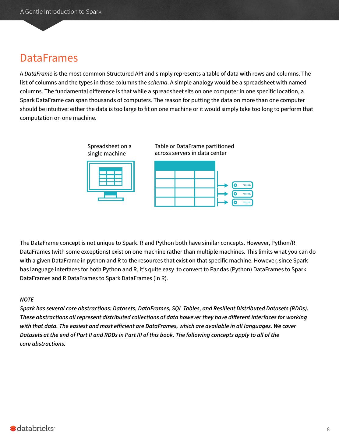
8 .A Gentle Introduction to Spark DataFrames A DataFrame is the most common Structured API and simply represents a table of data with rows and columns. The list of columns and the types in those columns the schema. A simple analogy would be a spreadsheet with named columns. The fundamental difference is that while a spreadsheet sits on one computer in one specific location, a Spark DataFrame can span thousands of computers. The reason for putting the data on more than one computer should be intuitive: either the data is too large to fit on one machine or it would simply take too long to perform that computation on one machine. Spreadsheet on a Table or DataFrame partitioned single machine across servers in data center The DataFrame concept is not unique to Spark. R and Python both have similar concepts. However, Python/R DataFrames (with some exceptions) exist on one machine rather than multiple machines. This limits what you can do with a given DataFrame in python and R to the resources that exist on that specific machine. However, since Spark has language interfaces for both Python and R, it’s quite easy to convert to Pandas (Python) DataFrames to Spark DataFrames and R DataFrames to Spark DataFrames (in R). NOTE Spark has several core abstractions: Datasets, DataFrames, SQL Tables, and Resilient Distributed Datasets (RDDs). These abstractions all represent distributed collections of data however they have different interfaces for working with that data. The easiest and most efficient are DataFrames, which are available in all languages. We cover Datasets at the end of Part II and RDDs in Part III of this book. The following concepts apply to all of the core abstractions. 8 

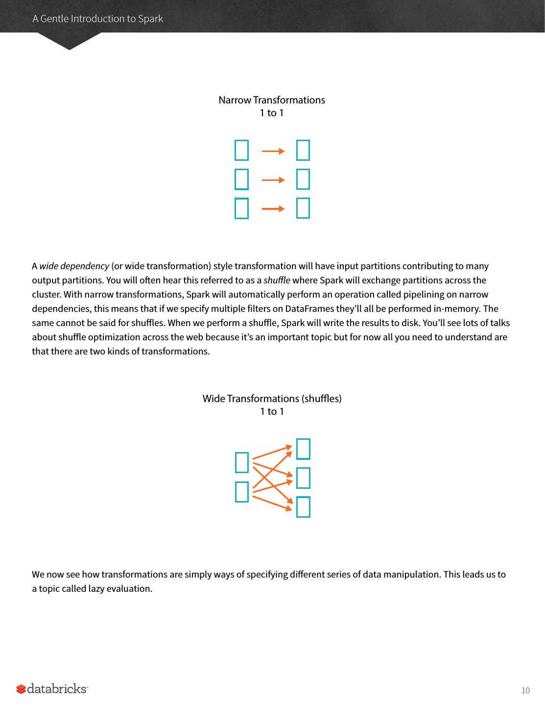
9 .A Gentle Introduction to Spark Partitions In order to allow every executor to perform work in parallel, Spark breaks up the data into chunks, called partitions. A partition is a collection of rows that sit on one physical machine in our cluster. A DataFrame’s partitions represent how the data is physically distributed across your cluster of machines during execution. If you have one partition, Spark will only have a parallelism of one even if you have thousands of executors. If you have many partitions, but only one executor Spark will still only have a parallelism of one because there is only one computation resource. An important thing to note, is that with DataFrames, we do not (for the most part) manipulate partitions manually (on an individual basis). We simply specify high level transformations of data in the physical partitions and Spark determines how this work will actually execute on the cluster. Lower level APIs do exist (via the Resilient Distributed Datasets interface) and we cover those in Part III of this book. Transformations In Spark, the core data structures are immutable meaning they cannot be changed once created. This might seem like a strange concept at first, if you cannot change it, how are you supposed to use it? In order to "change" a DataFrame you will have to instruct Spark how you would like to modify the DataFrame you have into the one that you want. These instructions are called transformations. Let’s perform a simple transformation to find all even numbers in our currentDataFrame. %scala val divisBy2 = myRange.where("number % 2 = 0") %python divisBy2 = myRange.where("number % 2 = 0") You will notice that these return no output, that’s because we only specified an abstract transformation and Spark will not act on transformations until we call an action, discussed shortly. Transformations are the core of how you will be expressing your business logic using Spark. There are two types of transformations, those that specify narrow dependencies and those that specify wide dependencies. Transformations consisting of narrow dependenciess (we’ll call them narrow transformations) are those where each input partition will contribute to only one output partition. In the preceding code snippet, our where statement specifies a narrow dependency, where only one partition contributes to at most one output partition. 9 

10 .A Gentle Introduction to Spark Narrow Transformations 1 to 1 A wide dependency (or wide transformation) style transformation will have input partitions contributing to many output partitions. You will often hear this referred to as a shuffle where Spark will exchange partitions across the cluster. With narrow transformations, Spark will automatically perform an operation called pipelining on narrow dependencies, this means that if we specify multiple filters on DataFrames they’ll all be performed in-memory. The same cannot be said for shuffles. When we perform a shuffle, Spark will write the results to disk. You’ll see lots of talks about shuffle optimization across the web because it’s an important topic but for now all you need to understand are that there are two kinds of transformations. Wide Transformations (shuffles) 1 to 1 We now see how transformations are simply ways of specifying different series of data manipulation. This leads us to a topic called lazy evaluation. 10 

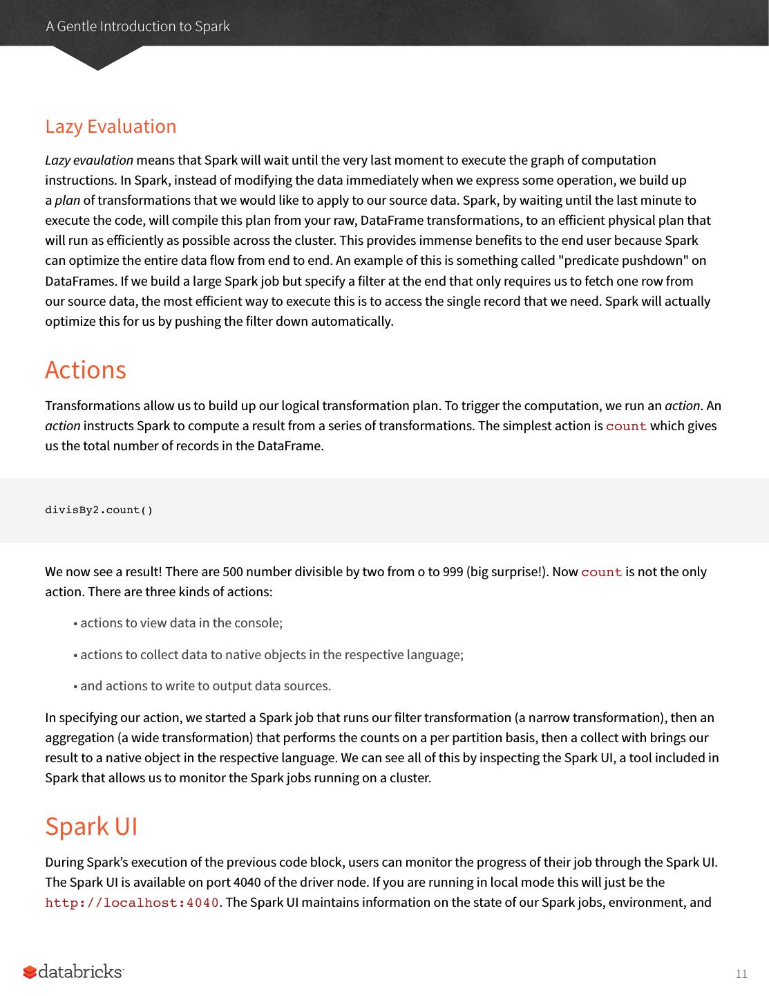
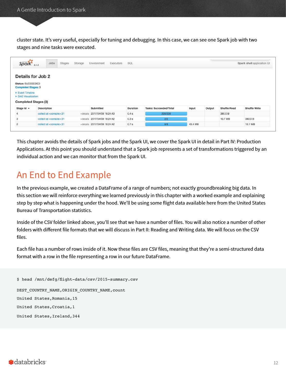
11 .A Gentle Introduction to Spark Lazy Evaluation Lazy evaulation means that Spark will wait until the very last moment to execute the graph of computation instructions. In Spark, instead of modifying the data immediately when we express some operation, we build up a plan of transformations that we would like to apply to our source data. Spark, by waiting until the last minute to execute the code, will compile this plan from your raw, DataFrame transformations, to an efficient physical plan that will run as efficiently as possible across the cluster. This provides immense benefits to the end user because Spark can optimize the entire data flow from end to end. An example of this is something called "predicate pushdown" on DataFrames. If we build a large Spark job but specify a filter at the end that only requires us to fetch one row from our source data, the most efficient way to execute this is to access the single record that we need. Spark will actually optimize this for us by pushing the filter down automatically. Actions Transformations allow us to build up our logical transformation plan. To trigger the computation, we run an action. An action instructs Spark to compute a result from a series of transformations. The simplest action is count which gives us the total number of records in the DataFrame. divisBy2.count() We now see a result! There are 500 number divisible by two from o to 999 (big surprise!). Now count is not the only action. There are three kinds of actions: • actions to view data in the console; • actions to collect data to native objects in the respective language; • and actions to write to output data sources. In specifying our action, we started a Spark job that runs our filter transformation (a narrow transformation), then an aggregation (a wide transformation) that performs the counts on a per partition basis, then a collect with brings our result to a native object in the respective language. We can see all of this by inspecting the Spark UI, a tool included in Spark that allows us to monitor the Spark jobs running on a cluster. Spark UI During Spark’s execution of the previous code block, users can monitor the progress of their job through the Spark UI. The Spark UI is available on port 4040 of the driver node. If you are running in local mode this will just be the http://localhost:4040. The Spark UI maintains information on the state of our Spark jobs, environment, and 11 

12 .A Gentle Introduction to Spark cluster state. It’s very useful, especially for tuning and debugging. In this case, we can see one Spark job with two stages and nine tasks were executed. This chapter avoids the details of Spark jobs and the Spark UI, we cover the Spark UI in detail in Part IV: Production Applications. At this point you should understand that a Spark job represents a set of transformations triggered by an individual action and we can monitor that from the Spark UI. An End to End Example In the previous example, we created a DataFrame of a range of numbers; not exactly groundbreaking big data. In this section we will reinforce everything we learned previously in this chapter with a worked example and explaining step by step what is happening under the hood. We’ll be using some flight data available here from the United States Bureau of Transportation statistics. Inside of the CSV folder linked above, you’ll see that we have a number of files. You will also notice a number of other folders with different file formats that we will discuss in Part II: Reading and Writing data. We will focus on the CSV files. Each file has a number of rows inside of it. Now these files are CSV files, meaning that they’re a semi-structured data format with a row in the file representing a row in our future DataFrame. $ head /mnt/defg/flight-data/csv/2015-summary.csv DEST_COUNTRY_NAME,ORIGIN_COUNTRY_NAME,count United States,Romania,15 United States,Croatia,1 United States,Ireland,344 12 

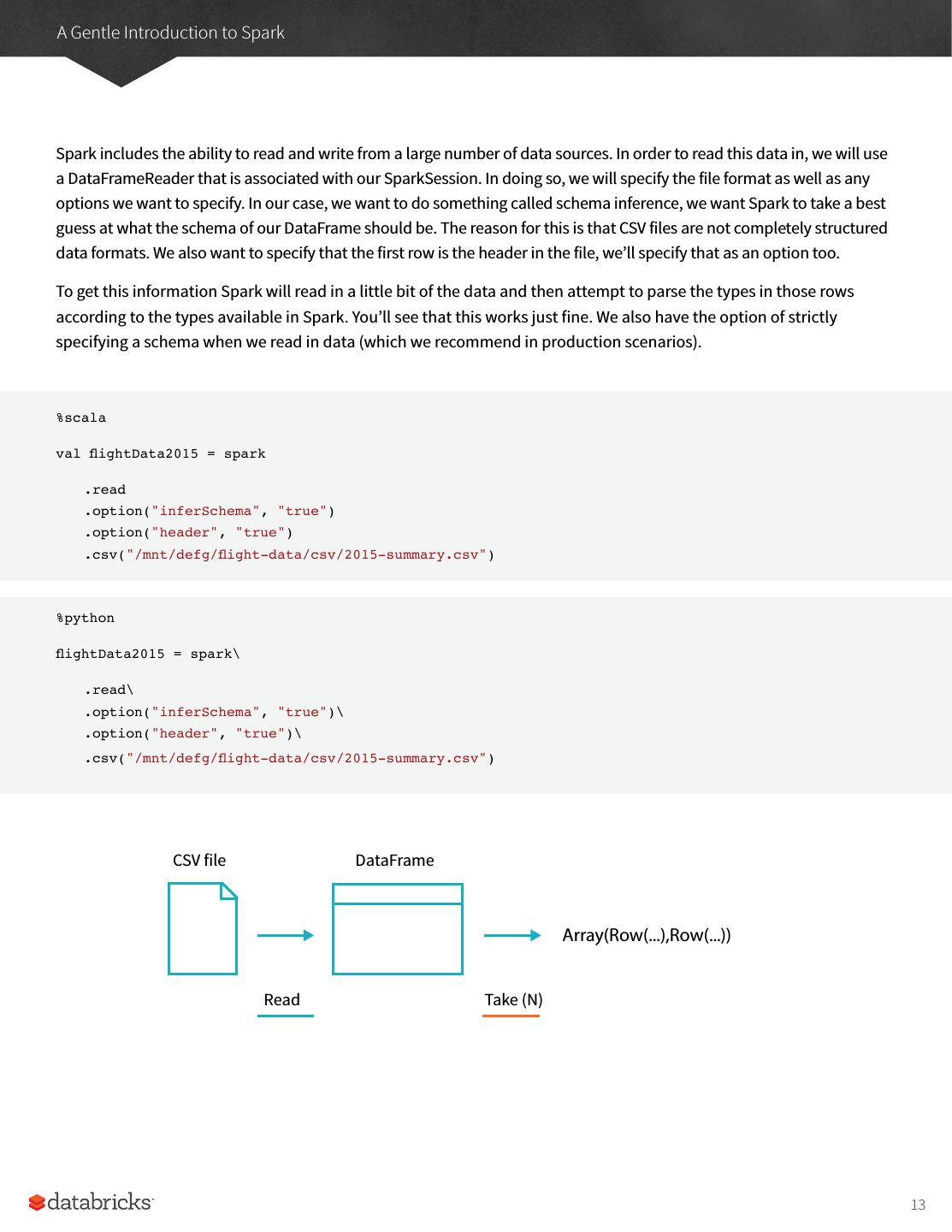
13 .A Gentle Introduction to Spark Spark includes the ability to read and write from a large number of data sources. In order to read this data in, we will use a DataFrameReader that is associated with our SparkSession. In doing so, we will specify the file format as well as any options we want to specify. In our case, we want to do something called schema inference, we want Spark to take a best guess at what the schema of our DataFrame should be. The reason for this is that CSV files are not completely structured data formats. We also want to specify that the first row is the header in the file, we’ll specify that as an option too. To get this information Spark will read in a little bit of the data and then attempt to parse the types in those rows according to the types available in Spark. You’ll see that this works just fine. We also have the option of strictly specifying a schema when we read in data (which we recommend in production scenarios). %scala val flightData2015 = spark .read .option("inferSchema", "true") .option("header", "true") .csv("/mnt/defg/flight-data/csv/2015-summary.csv") %python flightData2015 = spark\ .read\ .option("inferSchema", "true")\ .option("header", "true")\ .csv("/mnt/defg/flight-data/csv/2015-summary.csv") CSV file DataFrame Array(Row(...),Row(...)) Read Take (N) 13 

14 .A Gentle Introduction to Spark Each of these DataFrames (in Scala and Python) each have a set of columns with an unspecified number of rows. The reason the number of rows is "unspecified" is because reading data is a transformation, and is therefore a lazy operation. Spark only peeked at a couple of rows of data to try to guess what types each column should be. If we perform the take action on the DataFrame, we will be able to see the same results that we saw before when we used the command line. flightData2015.take(3) Array([United States,Romania,15], [United States,Croatia... Let’s specify some more transformations! Now we will sort our data according to the count column which is an integer type. NOTE Remember, the sort does not modify the DataFrame. We use the sort is a transformation that returns a new DataFrame by transforming the previous DataFrame. Let’s illustrate what’s happening when we call take on that resulting DataFrame. CSV file DataFrame DataFrame Array(...) Read Sort take(3) (Narrow) (Wide) (Wide) Nothing hpapens to the data when we call sort because it’s just a transformation. However, we can see that Spark is building up a plan for how it will execute this across the cluster by looking at the explain plan. We can call explain on any DataFrame object to see the DataFrame’s lineage (or how Spark will execute this query). flightData2015.sort("count").explain() Congratulations, you’ve just read your first explain plan! Explain plans are a bit arcane, but with a bit of practice it becomes second nature. Explain plans can be read from top to bottom, the top being the end result and the 14 

15 .A Gentle Introduction to Spark bottom being the source(s) of data. In our case, just take a look at the first keywords. You will see "sort", "exchange", and "FileScan". That’s because the sort of our data is actually a wide transformation because rows will have to be compared with one another. Don’t worry too much about understanding everything about explain plans at this point, they can just be helpful tools for debugging and improving your knowledge as you progress with Spark. Now, just like we did before, we can specify an action in order to kick off this plan. However before doing that, we’re going to set a configuration. By default, when we perform a shuffle Spark will output two hundred shuffle partitions. We will set this value to five in order to reduce the number of the output partitions from the shuffle from two hundred to five. spark.conf.set("spark.sql.shuffle.partitions", "5") flightData2015.sort("count").take(2) ... Array([United States,Singapore,1], [Moldova,United States,1]) This operation is illustrated in the following image. You’ll notice that in addition to the logical transformations, we include the physical partition count as well. CSV file DataFrame DataFrame Array(...) Read Sort take(3) (Narrow) (Wide) (Wide) 1 Partition 5 Partitions The logical plan of transformations that we build up defines a lineage for the DataFrame so that at any given point in time Spark knows how to recompute any partition by performing all of the operations it had before on the same input data. This sits at the heart of Spark’s programming model, functional programming where the same inputs always result in the same outputs when the transformations on that data stay constant. 15 

16 .A Gentle Introduction to Spark We do not manipulate the physical data, but rather configure physical execution characteristics through things like the shuffle partitions parameter we set above. We got five output partitions because that’s what we changed the shuffle partition value to. You can change this to help control the physical execution characteristics of your Spark jobs. Go ahead and experiment with different values and see the number of partitions yourself. In experimenting with different values, you should see drastically different run times. Remeber that you can monitor the job progress by navigating to the Spark UI on port 4040 to see the physical and logical execution characteristics of our jobs. DataFrames and SQL We worked through a simple example in the previous example, let’s now work through a more complex example and follow along in both DataFrames and SQL. Spark the same transformations, regardless of the language, in the exact same way. You can express your business logic in SQL or DataFrames (either in R, Python, Scala, or Java) and Spark will compile that logic down to an underlying plan (that we see in the explain plan) before actually executing your code. Spark SQL allows you as a user to register any DataFrame as a table or view (a temporary table) and query it using pure SQL. There is no performance difference between writing SQL queries or writing DataFrame code, they both "compile" to the same underlying plan that we specify in DataFrame code. Any DataFrame can be made into a table or view with one simple method call. %scala flightData2015.createOrReplaceTempView("flight_data_2015") %python flightData2015.createOrReplaceTempView("flight_data_2015") Now we can query our data in SQL. To execute a SQL query, we’ll use the spark.sql function (remember spark is our SparkSession variable?) that conveniently, returns a new DataFrame. While this may seem a bit circular in logic - that a SQL query against a DataFrame returns another DataFrame, it’s actually quite powerful. As a user, you can specify transformations in the manner most convenient to you at any given point in time and not have to trade any efficiency to do so! To understand that this is happening, let’s take a look at two explain plans. 16 

17 .A Gentle Introduction to Spark %scala val sqlWay = spark.sql(""" SELECT DEST_COUNTRY_NAME, count(1) FROM flight_data_2015 GROUP BY DEST_COUNTRY_NAME """) val dataFrameWay = flightData2015 .groupBy(‘DEST_COUNTRY_NAME) .count() sqlWay.explain dataFrameWay.explain %python sqlWay = spark.sql(""" SELECT DEST_COUNTRY_NAME, count(1) FROM flight_data_2015 GROUP BY DEST_COUNTRY_NAME """) dataFrameWay = flightData2015\ .groupBy("DEST_COUNTRY_NAME")\ .count() sqlWay.explain() dataFrameWay.explain() == Physical Plan == *HashAggregate(keys=[DEST_COUNTRY_NAME#182], functions=[count(1)]) +- Exchange hashpartitioning(DEST_COUNTRY_NAME#182, 5) +- *HashAggregate(keys=[DEST_COUNTRY_NAME#182], functions=[partial_count(1)]) +- *FileScan csv [DEST_COUNTRY_NAME#182] ... == Physical Plan == *HashAggregate(keys=[DEST_COUNTRY_NAME#182], functions=[count(1)]) +- Exchange hashpartitioning(DEST_COUNTRY_NAME#182, 5) +- *HashAggregate(keys=[DEST_COUNTRY_NAME#182], functions=[partial_count(1)]) +- *FileScan csv [DEST_COUNTRY_NAME#182] ... 17 

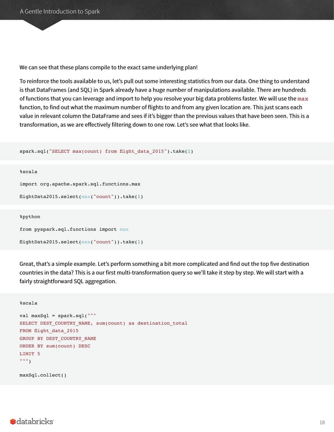
18 .A Gentle Introduction to Spark We can see that these plans compile to the exact same underlying plan! To reinforce the tools available to us, let’s pull out some interesting statistics from our data. One thing to understand is that DataFrames (and SQL) in Spark already have a huge number of manipulations available. There are hundreds of functions that you can leverage and import to help you resolve your big data problems faster. We will use the max function, to find out what the maximum number of flights to and from any given location are. This just scans each value in relevant column the DataFrame and sees if it’s bigger than the previous values that have been seen. This is a transformation, as we are effectively filtering down to one row. Let’s see what that looks like. spark.sql("SELECT max(count) from flight_data_2015").take(1) %scala import org.apache.spark.sql.functions.max flightData2015.select(max("count")).take(1) %python from pyspark.sql.functions import max flightData2015.select(max("count")).take(1) Great, that’s a simple example. Let’s perform something a bit more complicated and find out the top five destination countries in the data? This is a our first multi-transformation query so we’ll take it step by step. We will start with a fairly straightforward SQL aggregation. %scala val maxSql = spark.sql(""" SELECT DEST_COUNTRY_NAME, sum(count) as destination_total FROM flight_data_2015 GROUP BY DEST_COUNTRY_NAME ORDER BY sum(count) DESC LIMIT 5 """) maxSql.collect() 18 

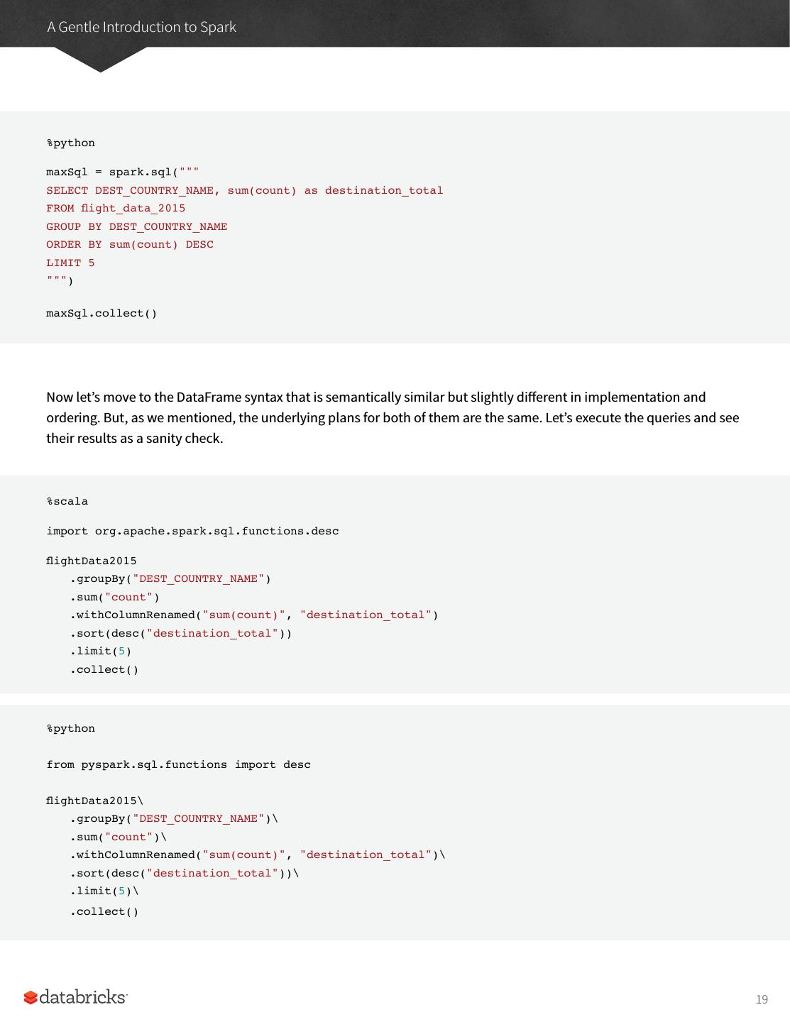
19 .A Gentle Introduction to Spark %python maxSql = spark.sql(""" SELECT DEST_COUNTRY_NAME, sum(count) as destination_total FROM flight_data_2015 GROUP BY DEST_COUNTRY_NAME ORDER BY sum(count) DESC LIMIT 5 """) maxSql.collect() Now let’s move to the DataFrame syntax that is semantically similar but slightly different in implementation and ordering. But, as we mentioned, the underlying plans for both of them are the same. Let’s execute the queries and see their results as a sanity check. %scala import org.apache.spark.sql.functions.desc flightData2015 .groupBy("DEST_COUNTRY_NAME") .sum("count") .withColumnRenamed("sum(count)", "destination_total") .sort(desc("destination_total")) .limit(5) .collect() %python from pyspark.sql.functions import desc flightData2015\ .groupBy("DEST_COUNTRY_NAME")\ .sum("count")\ .withColumnRenamed("sum(count)", "destination_total")\ .sort(desc("destination_total"))\ .limit(5)\ .collect() 19 

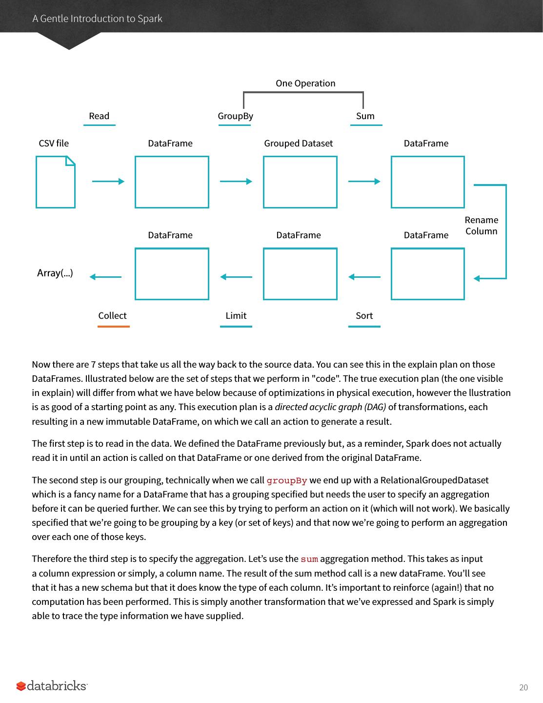
20 .A Gentle Introduction to Spark One Operation Read GroupBy Sum CSV file DataFrame Grouped Dataset DataFrame Rename DataFrame DataFrame DataFrame Column Array(...) Collect Limit Sort Now there are 7 steps that take us all the way back to the source data. You can see this in the explain plan on those DataFrames. Illustrated below are the set of steps that we perform in "code". The true execution plan (the one visible in explain) will differ from what we have below because of optimizations in physical execution, however the llustration is as good of a starting point as any. This execution plan is a directed acyclic graph (DAG) of transformations, each resulting in a new immutable DataFrame, on which we call an action to generate a result. The first step is to read in the data. We defined the DataFrame previously but, as a reminder, Spark does not actually read it in until an action is called on that DataFrame or one derived from the original DataFrame. The second step is our grouping, technically when we call groupBy we end up with a RelationalGroupedDataset which is a fancy name for a DataFrame that has a grouping specified but needs the user to specify an aggregation before it can be queried further. We can see this by trying to perform an action on it (which will not work). We basically specified that we’re going to be grouping by a key (or set of keys) and that now we’re going to perform an aggregation over each one of those keys. Therefore the third step is to specify the aggregation. Let’s use the sum aggregation method. This takes as input a column expression or simply, a column name. The result of the sum method call is a new dataFrame. You’ll see that it has a new schema but that it does know the type of each column. It’s important to reinforce (again!) that no computation has been performed. This is simply another transformation that we’ve expressed and Spark is simply able to trace the type information we have supplied. 20 

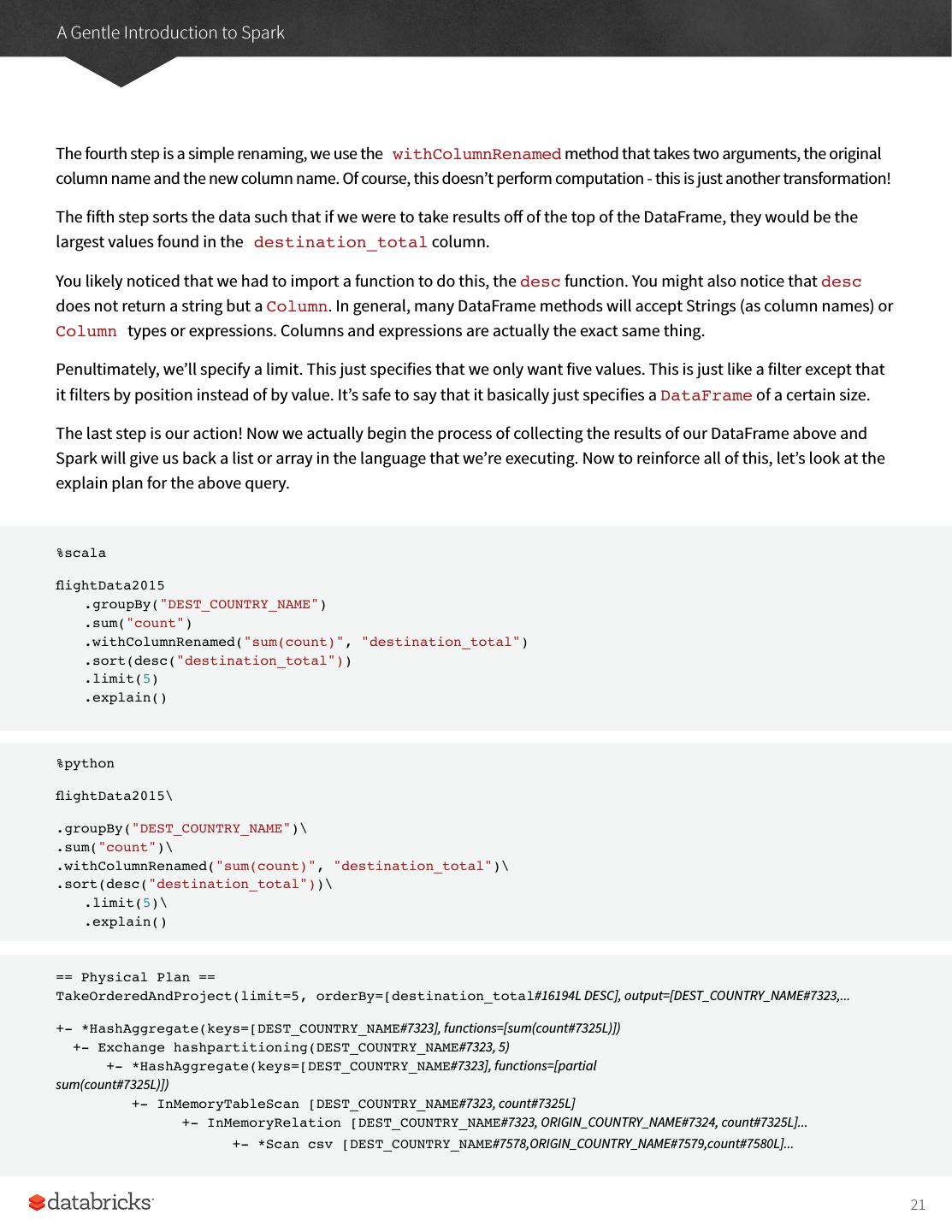
21 .A Gentle Introduction to Spark The fourth step is a simple renaming, we use the withColumnRenamed method that takes two arguments, the original column name and the new column name. Of course, this doesn’t perform computation - this is just another transformation! The fifth step sorts the data such that if we were to take results off of the top of the DataFrame, they would be the largest values found in the destination_total column. You likely noticed that we had to import a function to do this, the desc function. You might also notice that desc does not return a string but a Column. In general, many DataFrame methods will accept Strings (as column names) or Column types or expressions. Columns and expressions are actually the exact same thing. Penultimately, we’ll specify a limit. This just specifies that we only want five values. This is just like a filter except that it filters by position instead of by value. It’s safe to say that it basically just specifies a DataFrame of a certain size. The last step is our action! Now we actually begin the process of collecting the results of our DataFrame above and Spark will give us back a list or array in the language that we’re executing. Now to reinforce all of this, let’s look at the explain plan for the above query. %scala flightData2015 .groupBy("DEST_COUNTRY_NAME") .sum("count") .withColumnRenamed("sum(count)", "destination_total") .sort(desc("destination_total")) .limit(5) .explain() %python flightData2015\ .groupBy("DEST_COUNTRY_NAME")\ .sum("count")\ .withColumnRenamed("sum(count)", "destination_total")\ .sort(desc("destination_total"))\ .limit(5)\ .explain() == Physical Plan == TakeOrderedAndProject(limit=5, orderBy=[destination_total#16194L DESC], output=[DEST_COUNTRY_NAME#7323,... +- *HashAggregate(keys=[DEST_COUNTRY_NAME#7323], functions=[sum(count#7325L)]) +- Exchange hashpartitioning(DEST_COUNTRY_NAME#7323, 5) +- *HashAggregate(keys=[DEST_COUNTRY_NAME#7323], functions=[partial sum(count#7325L)]) +- InMemoryTableScan [DEST_COUNTRY_NAME#7323, count#7325L] +- InMemoryRelation [DEST_COUNTRY_NAME#7323, ORIGIN_COUNTRY_NAME#7324, count#7325L]... +- *Scan csv [DEST_COUNTRY_NAME#7578,ORIGIN_COUNTRY_NAME#7579,count#7580L]... 21 

22 .While this explain plan doesn’t match our exact "conceptual plan" all of the pieces are there. You can see the limit statement as well as the orderBy (in the first line). You can also see how our aggregation happens in two phases, in the partial_sum calls. This is because summing a list of numbers is commutative and Spark can perform the sum, partition by partition. Of course we can see how we read in the DataFrame as well. Naturally, we don’t always have to collect the data. We can also write it out to any data source that Spark supports. For instance, let’s say that we wanted to store the information in a database like PostgreSQL or write them out to another file. 22 

23 .A Tour of Spark’s Toolset In the previous chapter we introduced Spark’s core concepts, like transformations and actions, in the context of Spark’s Structured APIs. These simple conceptual building blocks are the foundation of Apache Spark’s vast ecosystem of tools and libraries. Spark is composed of the simple primitives, the lower level APIs and the Structured APIs, then a series of "standard libraries" included in Spark. Advanced analytics Ecosystem Structured ML graph + streaming Deep learning Packages Structured APIs Datasets DataFrames SQL Low level APIs Distributed variables RDDs Developers use these tools for a variety of different tasks, from graph analysis and machine learning to streaming and integrations with a host of libraries and databases. This chapter will present a whirlwind tour of much of what Spark has to offer. Each section in this chapter are elaborated upon by other parts of this book, this chapter is simply here to show you what’s possible. This chapter will cover: • Production applications with spark-submit, • Datasets: structured and type safe APIs, • Structured Streaming, • Machine learning and advanced analytics, 23 

24 .A Tour of Spark’s Toolset • Spark’s lower level APIs, • SparkR, • Spark’s package ecosystem. The entire book covers these topics in depth, the goal of this chapter is simply to provide a whirlwind tour of Spark. Once you’ve gotten the tour, you’ll be able to jump to many different parts of the book to find answers to your questions about particular topics. This chapter aims for breadth, instead of depth. Let’s get started! Production Applications Spark makes it easy to make simple to reason about and simple to evolve big data programs. Spark also makes it easy to turn in your interactive exploration into production applications with a tool called spark-submit that is included in the core of Spark. spark-submit does one thing, it allows you to submit your applications to a currently managed cluster to run. When you submit this, the application will run until the application exists or errors. You can do this with all of Spark’s support cluster managers including Standalone, Mesos, and YARN. In the process of doing so, you have a number of knobs that you can turn and control to specify the resources this application has as well, how it should be run, and the parameters for your specific application. You can write these production applications in any of Spark’s supported languages and then submit those applications for execution. The simplest example is one that you can do on your local machine by running the following command line snippet on your local machine in the directory into which you downloaded Spark. ./bin/spark-submit \ --class org.apache.spark.examples.SparkPi \ --master local \ ./examples/jars/spark-examples_2.11-2.2.0.jar 10 What this will do is calculate the digits of pi to a certain level of estimation. What we’ve done here is specified that we want to run it on our local machine, specified which class and which jar we would like to run as well as any command line arguments to that particular class. We can do this in Python with the following command line arguments. 24 

25 .A Tour of Spark’s Toolset ./bin/spark-submit \ --master local \ ./examples/src/main/python/pi.py 10 By swapping out the path to the file and the cluster configurations, we can write and run production applications. Now Spark provides a lot more than just DataFrames that we can run as production applications. The rest of this chapter will walk through several different APIs that we can leverage to run all sorts of production applications. Datasets: Type-Safe Structured APIs The next topic we’ll cover is a type-safe version of Spark’s structured API for Java and Scala, called Datasets. This API is not available in Python and R, because those are dynamically typed languages, but it is a powerful tool for writing large applications in Scala and Java. Recall that DataFrames, which we saw earlier, are a distributed collection of objects of type Row, which can hold various types of tabular data. The Dataset API allows users to assign a Java class to the records inside a DataFrame, and manipulate it as a collection of typed objects, similar to a Java ArrayList or Scala Seq. The APIs available on Datasets are type-safe, meaning that you cannot accidentally view the objects in a Dataset as being of another class than the class you put in initially. This makes Datasets especially attractive for writing large applications where multiple software engineers must interact through well-defined interfaces. The Dataset class is parametrized with the type of object contained inside: Dataset<T> in Java and Dataset[T] in Scala. As of Spark 2.0, the types T supported are all classes following the JavaBean pattern in Java, and case classes in Scala. These types are restricted because Spark needs to be able to automatically analyze the type T and create an appropriate schema for the tabular data inside your Dataset. The awesome thing about Datasets is that we can use them only when we need or want to. For instance, in the follow example I’ll define my own object and manipulate it via arbitrary map and filter functions. Once we’ve performed our manipulations, Spark can automatically turn it back into a DataFrame and we can manipulate it further using the hundreds of functions that Spark includes. This makes it easy to drop down to lower level, perform type-safe coding when necessary, and move higher up to SQL for more rapid analysis. We cover this material extensively in the next part of this book, but here is a small example showing how we can use both type-safe functions and DataFrame-like SQL expressions to quickly write business logic. 25 

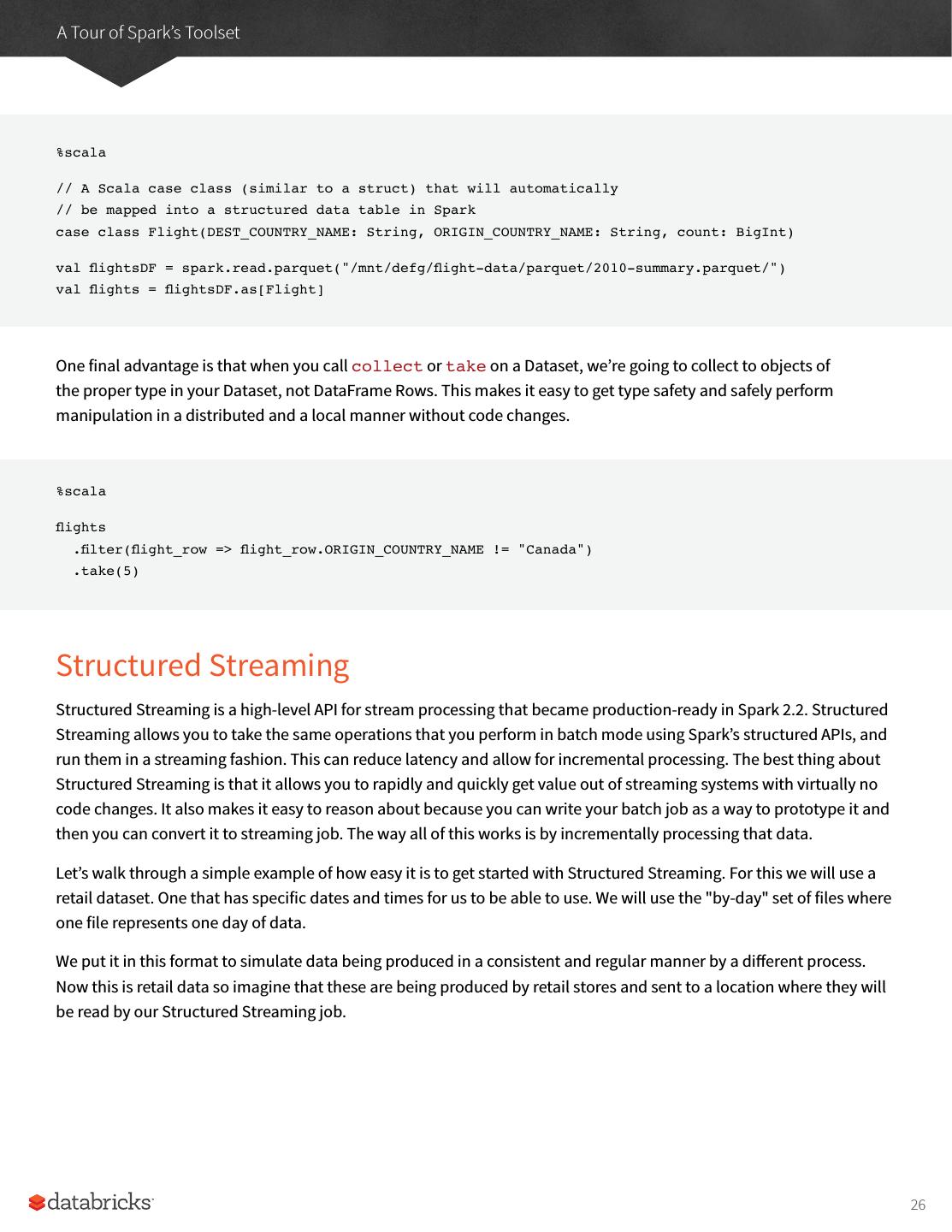
26 .A Tour of Spark’s Toolset %scala // A Scala case class (similar to a struct) that will automatically // be mapped into a structured data table in Spark case class Flight(DEST_COUNTRY_NAME: String, ORIGIN_COUNTRY_NAME: String, count: BigInt) val flightsDF = spark.read.parquet("/mnt/defg/flight-data/parquet/2010-summary.parquet/") val flights = flightsDF.as[Flight] One final advantage is that when you call collect or take on a Dataset, we’re going to collect to objects of the proper type in your Dataset, not DataFrame Rows. This makes it easy to get type safety and safely perform manipulation in a distributed and a local manner without code changes. %scala flights .filter(flight_row => flight_row.ORIGIN_COUNTRY_NAME != "Canada") .take(5) Structured Streaming Structured Streaming is a high-level API for stream processing that became production-ready in Spark 2.2. Structured Streaming allows you to take the same operations that you perform in batch mode using Spark’s structured APIs, and run them in a streaming fashion. This can reduce latency and allow for incremental processing. The best thing about Structured Streaming is that it allows you to rapidly and quickly get value out of streaming systems with virtually no code changes. It also makes it easy to reason about because you can write your batch job as a way to prototype it and then you can convert it to streaming job. The way all of this works is by incrementally processing that data. Let’s walk through a simple example of how easy it is to get started with Structured Streaming. For this we will use a retail dataset. One that has specific dates and times for us to be able to use. We will use the "by-day" set of files where one file represents one day of data. We put it in this format to simulate data being produced in a consistent and regular manner by a different process. Now this is retail data so imagine that these are being produced by retail stores and sent to a location where they will be read by our Structured Streaming job. 26 

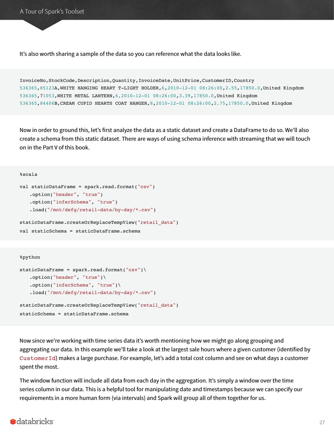
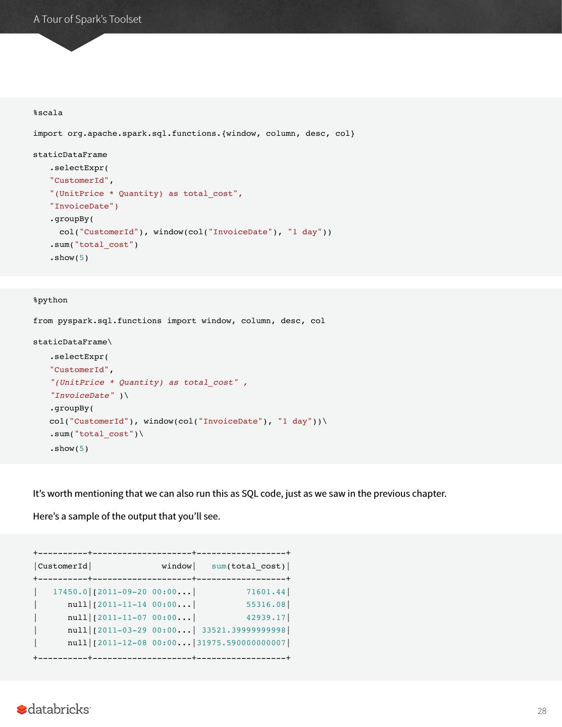
27 .A Tour of Spark’s Toolset It’s also worth sharing a sample of the data so you can reference what the data looks like. InvoiceNo,StockCode,Description,Quantity,InvoiceDate,UnitPrice,CustomerID,Country 536365,85123A,WHITE HANGING HEART T-LIGHT HOLDER,6,2010-12-01 08:26:00,2.55,17850.0,United Kingdom 536365,71053,WHITE METAL LANTERN,6,2010-12-01 08:26:00,3.39,17850.0,United Kingdom 536365,84406B,CREAM CUPID HEARTS COAT HANGER,8,2010-12-01 08:26:00,2.75,17850.0,United Kingdom Now in order to ground this, let’s first analyze the data as a static dataset and create a DataFrame to do so. We’ll also create a schema from this static dataset. There are ways of using schema inference with streaming that we will touch on in the Part V of this book. %scala val staticDataFrame = spark.read.format("csv") .option("header", "true") .option("inferSchema", "true") .load("/mnt/defg/retail-data/by-day/*.csv") staticDataFrame.createOrReplaceTempView("retail_data") val staticSchema = staticDataFrame.schema %python staticDataFrame = spark.read.format("csv")\ .option("header", "true")\ .option("inferSchema", "true")\ .load("/mnt/defg/retail-data/by-day/*.csv") staticDataFrame.createOrReplaceTempView("retail_data") staticSchema = staticDataFrame.schema Now since we’re working with time series data it’s worth mentioning how we might go along grouping and aggregating our data. In this example we’ll take a look at the largest sale hours where a given customer (identified by CustomerId) makes a large purchase. For example, let’s add a total cost column and see on what days a customer spent the most. The window function will include all data from each day in the aggregation. It’s simply a window over the time series column in our data. This is a helpful tool for manipulating date and timestamps because we can specify our requirements in a more human form (via intervals) and Spark will group all of them together for us. 27 

28 .A Tour of Spark’s Toolset %scala import org.apache.spark.sql.functions.{window, column, desc, col} staticDataFrame .selectExpr( "CustomerId", "(UnitPrice * Quantity) as total_cost", "InvoiceDate") .groupBy( col("CustomerId"), window(col("InvoiceDate"), "1 day")) .sum("total_cost") .show(5) %python from pyspark.sql.functions import window, column, desc, col staticDataFrame\ .selectExpr( "CustomerId", "(UnitPrice * Quantity) as total_cost" , "InvoiceDate" )\ .groupBy( col("CustomerId"), window(col("InvoiceDate"), "1 day"))\ .sum("total_cost")\ .show(5) It’s worth mentioning that we can also run this as SQL code, just as we saw in the previous chapter. Here’s a sample of the output that you’ll see. +----------+--------------------+------------------+ |CustomerId| window| sum(total_cost)| +----------+--------------------+------------------+ | 17450.0|[2011-09-20 00:00...| 71601.44| | null|[2011-11-14 00:00...| 55316.08| | null|[2011-11-07 00:00...| 42939.17| | null|[2011-03-29 00:00...| 33521.39999999998| | null|[2011-12-08 00:00...|31975.590000000007| +----------+--------------------+------------------+ 28 

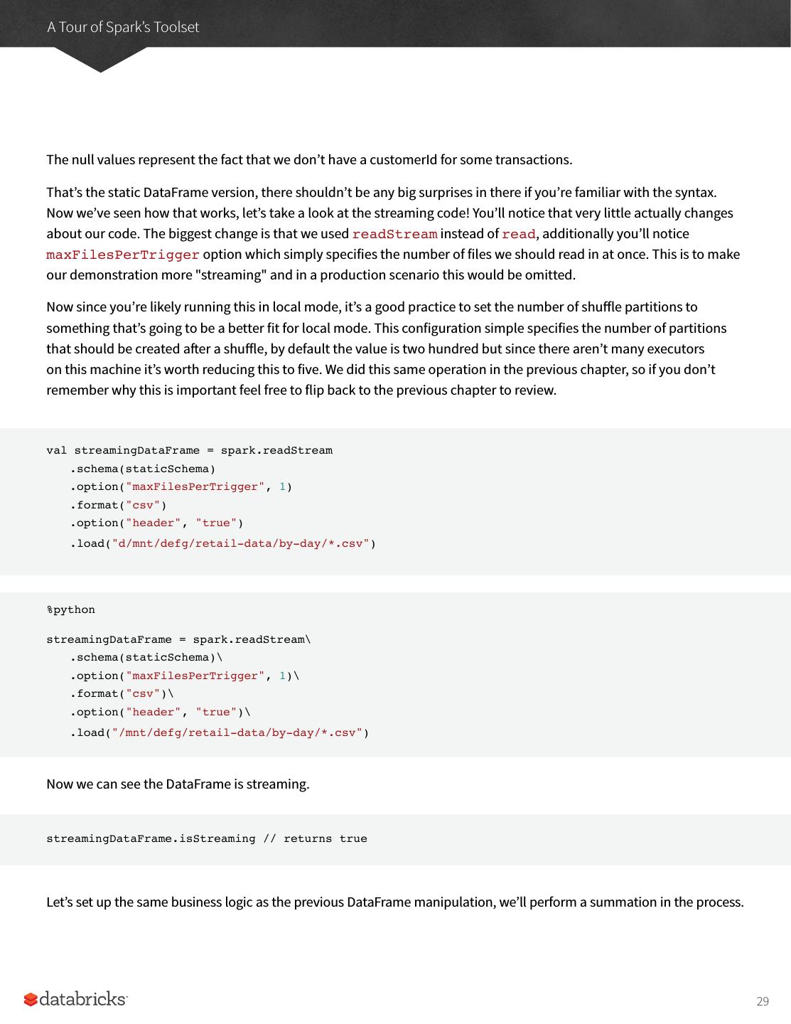
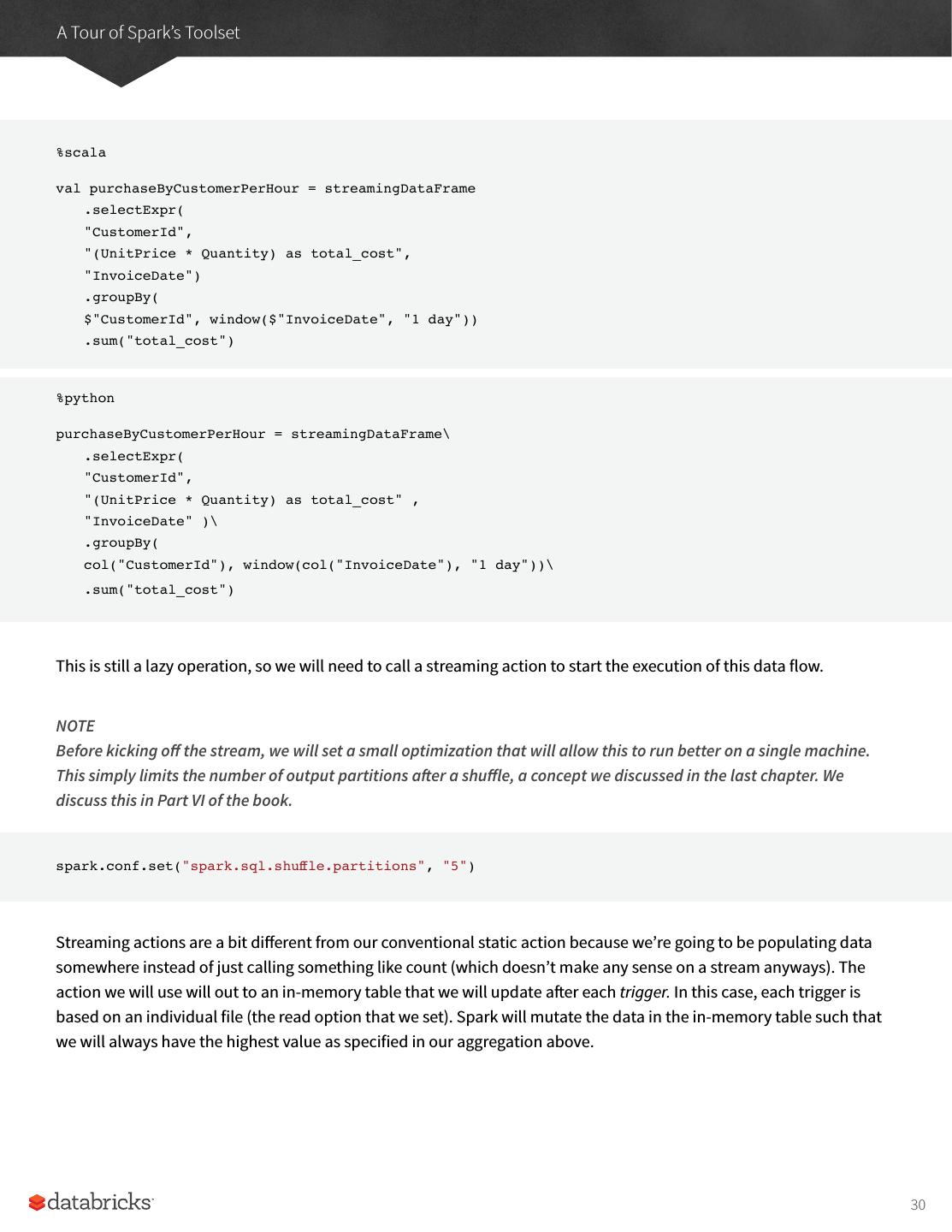
29 .A Tour of Spark’s Toolset The null values represent the fact that we don’t have a customerId for some transactions. That’s the static DataFrame version, there shouldn’t be any big surprises in there if you’re familiar with the syntax. Now we’ve seen how that works, let’s take a look at the streaming code! You’ll notice that very little actually changes about our code. The biggest change is that we used readStream instead of read, additionally you’ll notice maxFilesPerTrigger option which simply specifies the number of files we should read in at once. This is to make our demonstration more "streaming" and in a production scenario this would be omitted. Now since you’re likely running this in local mode, it’s a good practice to set the number of shuffle partitions to something that’s going to be a better fit for local mode. This configuration simple specifies the number of partitions that should be created after a shuffle, by default the value is two hundred but since there aren’t many executors on this machine it’s worth reducing this to five. We did this same operation in the previous chapter, so if you don’t remember why this is important feel free to flip back to the previous chapter to review. val streamingDataFrame = spark.readStream .schema(staticSchema) .option("maxFilesPerTrigger", 1) .format("csv") .option("header", "true") .load("d/mnt/defg/retail-data/by-day/*.csv") %python streamingDataFrame = spark.readStream\ .schema(staticSchema)\ .option("maxFilesPerTrigger", 1)\ .format("csv")\ .option("header", "true")\ .load("/mnt/defg/retail-data/by-day/*.csv") Now we can see the DataFrame is streaming. streamingDataFrame.isStreaming // returns true Let’s set up the same business logic as the previous DataFrame manipulation, we’ll perform a summation in the process. 29