Paper reading#3 基于近邻图的高维向量近似最近邻检索算法实验综述

1 . VLDB 2021 Experiment, Analysis & Benchmark A Comprehensive Survey and Experimental Comparison of Graph-Based Approximate Nearest Neighbor Search Mengzhao Wang, Xiaoliang Xu, Qiang Yue, Yuxiang Wang Hangzhou Dianzi University, China 

2 . Contents 2 p Background - Unstructured data; ANNS; Graph-based ANNS p Motivation - Why do we need a review of graph-based ANNS algorithms p Analysis - Macro and micro perspective p Evaluation - Index construction; Search; Components; Machine learning-based optimizations p Discussion - Recommendations; Guidelines; Improvement; Tendencies; Challenges 

3 . Background 3 p Unstructured data - Over 80% data growth is unstructured by 2025 ! - Embedding as a new source of data - Unstructured data is processed by vector similarity calculation https://ai.googleblog.com/2020/07/announcing-scann-efficient-vector.html 

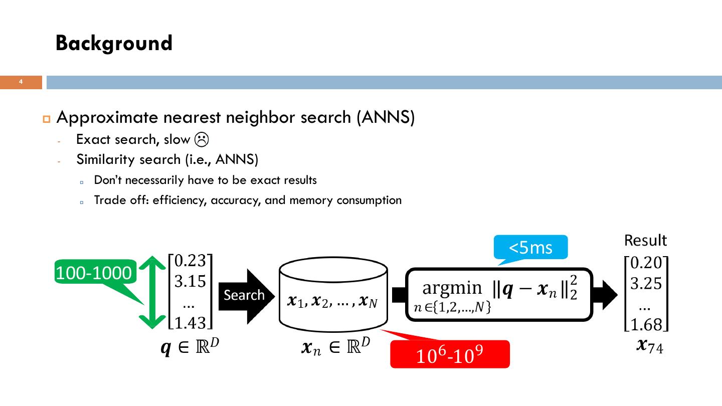
4 . Background 4 p Approximate nearest neighbor search (ANNS) - Exact search, slow - Similarity search (i.e., ANNS) p Don’t necessarily have to be exact results p Trade off: efficiency, accuracy, and memory consumption <5ms 100-1000 106-109 

5 . Background 5 p Different categories based on the index - Tree partitioning structures - Hashing-based techniques - Quantization-based methods - Proximity graph algorithms Best trade-off ! 

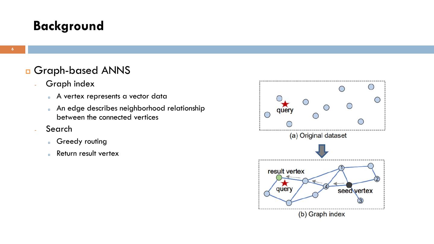
6 . Background 6 p Graph-based ANNS - Graph index p A vertex represents a vector data p An edge describes neighborhood relationship between the connected vertices - Search p Greedy routing p Return result vertex 

7 . Motivation 7 p Lack of a reasonable taxonomy and comparative analysis of inter-algorithm - Delaunay Graph (DG), Relative Neighborhood Graph (RNG), K-Nearest Neighbor Graph (KNNG), Minimum Spanning Tree (MST) - e.g., KNNG-based group: KGraph (WWW’11), SPTAG (ACM MM’12, CVPR’12, TPAMI’14) - e.g., RNG-based group: DPG (TKDE’19), HNSW (TPAMI’18) 

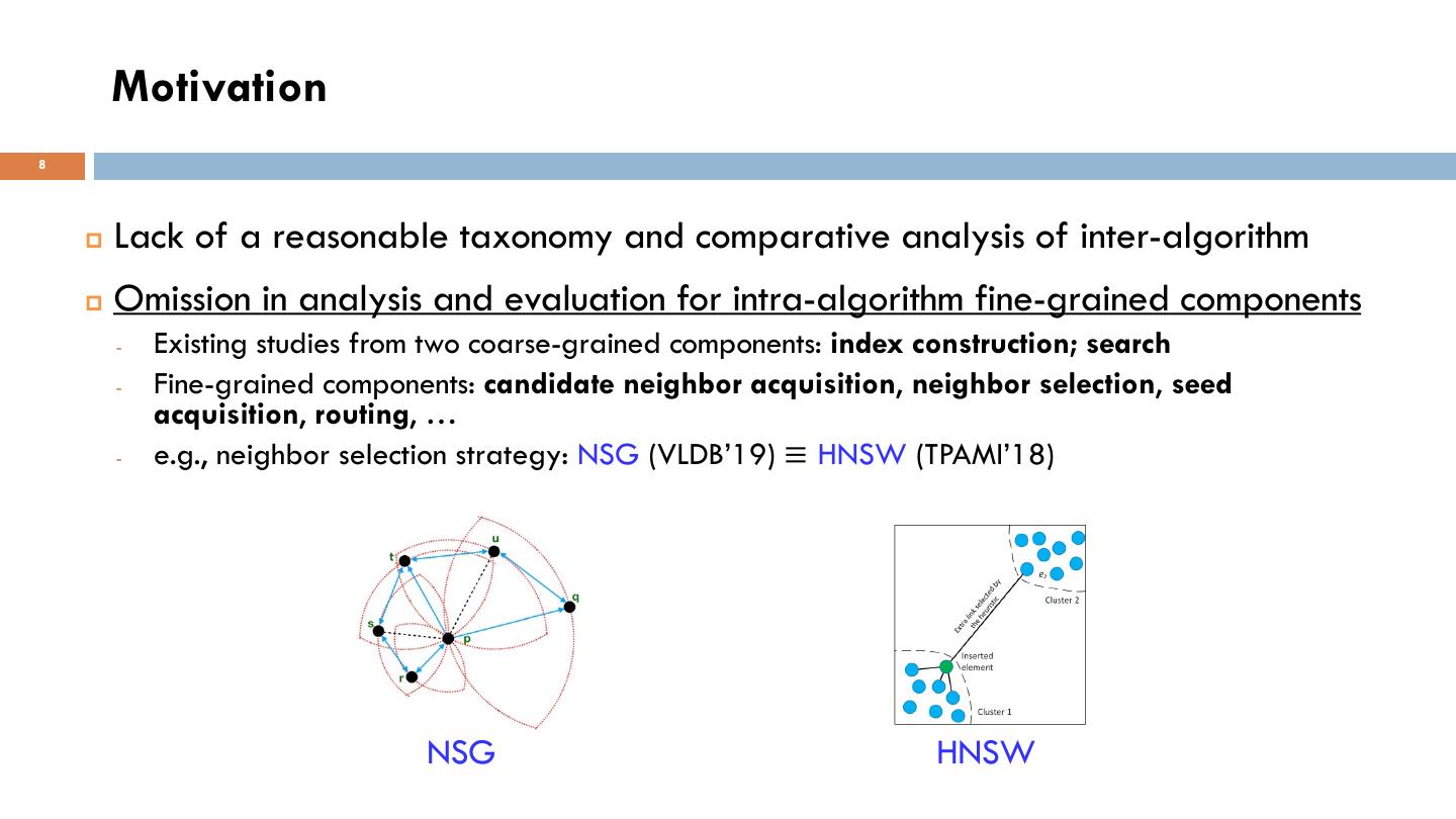
8 . Motivation 8 p Lack of a reasonable taxonomy and comparative analysis of inter-algorithm p Omission in analysis and evaluation for intra-algorithm fine-grained components - Existing studies from two coarse-grained components: index construction; search - Fine-grained components: candidate neighbor acquisition, neighbor selection, seed acquisition, routing, … - e.g., neighbor selection strategy: NSG (VLDB’19) ≡ HNSW (TPAMI’18) NSG HNSW 

9 . Motivation 9 p Lack of a reasonable taxonomy and comparative analysis of inter-algorithm p Omission in analysis and evaluation for intra-algorithm fine-grained components p Richer metrics are required for evaluating algorithms’ overall performance - Existing metrics: speedup vs recall, index construction efficiency, memory overhead - Some metrics indirectly affect above performance, such as graph quality, out-degree, … - e.g., higher graph quality does not necessarily achieve better search performance Graph quality: the percentage of vertices that are HNSW linked to their nearest neighbor on the graph DPG HNSW (TPAMI’18) : 63.3% DPG (TKDE’19) : 99.2% 

10 . Motivation 1 0 p Lack of a reasonable taxonomy and comparative analysis of inter-algorithm p Omission in analysis and evaluation for intra-algorithm fine-grained components p Richer metrics are required for evaluating algorithms’ overall performance p Diversified datasets are essential for algorithms’ scalability evaluation - Video, Audio, Text, Image, … - Dimensionality, cardinality, clusters, standard deviation of the distribution in each cluster - e.g., Speedup on different dataset: HNSW < NSG 125X on Msong, HNSW > NSG 80X on Crawl HNSW (TPAMI’18) NSG (VLDB’19) 

11 . Motivation 11 p Lack of a reasonable taxonomy and comparative analysis of inter-algorithm p Omission in analysis and evaluation for intra-algorithm fine-grained components p Richer metrics are required for evaluating algorithms’ overall performance p Diversified datasets are essential for algorithms’ scalability evaluation p Comparison of machine learning based optimizations - Recent trend of applying ML to graph-based ANNS algorithms (e.g., SIGMOD’20, ICML’20) 

12 . Analysis 12 p Macroscopic perspective (inter-algorithm) - 13 representative graph-based ANNS algorithms p KGraph (WWW’11), FANNG (CVPR’16), NSG (VLDB’19), NSSG (TPAMI’21), DPG (TKDE’19), Vamana (NeurIPS’19), EFANNA (CoRR’16), IEH (CYBERNETICS’14), HNSW (TPAMI’18), HCNNG (PR’19), NSW (IS’14), NGT (SISAP’16, CoRR’18), SPTAG (ACM MM’12, CVPR’12, TPAMI’14) - Base graphs for ANNS (taxonomy) p Delaunay graph (DG): ensure precise results; large search space; high construction complexity p Relative neighborhood graph (RNG): high search efficiency; high construction complexity p K-nearest neighbor graph (KNNG): memory friendly; unassured connectivity p Minimum spanning tree (MST): ensure connectivity; long search path 

13 . Analysis 13 p Macroscopic perspective (inter-algorithm) - Roadmap of graph-based ANNS algorithms - Optimizations of the algorithms for the base graphs p Improve index construction efficiency p Reduce index size p Improve search efficiency p Increase recall rate - Taxonomy of graph-based algorithms 

14 . Analysis 14 p Microcosmic perspective (intra-algorithm) - Graph-based ANNS algorithms follow a unified processing pipeline - Break down each algorithm into seven components (C1-C7) - Components for index construction (C1-C5) 

15 . Analysis 15 p Microcosmic perspective (intra-algorithm) - Graph-based ANNS algorithms follow a unified processing pipeline - Break down each algorithm into seven components (C1-C7) - Components for index construction (C1-C5) p Initialization p Candidate neighbor acquisition p Neighbor selection p Seed preprocessing p Connectivity 

16 . Analysis 16 p Microcosmic perspective (intra-algorithm) - Graph-based ANNS algorithms follow a unified processing pipeline - Break down each algorithm into seven components (C1-C7) - Components for index construction (C1-C5) p Initialization p Candidate neighbor acquisition p Neighbor selection p Seed preprocessing p Connectivity - Components for search (C6-C7) 

17 . Analysis 17 p Microcosmic perspective (intra-algorithm) - Graph-based ANNS algorithms follow a unified processing pipeline - Break down each algorithm into seven components (C1-C7) - Components for index construction (C1-C5) p Initialization p Candidate neighbor acquisition p Neighbor selection p Seed preprocessing p Connectivity - Components for search (C6-C7) BFS: best first search p Seed acquisition RS: range search p Routing GS: guided search 

18 . Experimental Overview 18 p Lack of a reasonable taxonomy and comparative analysis of inter-algorithm - Overall performance evaluation among 13 algorithms p Omission in analysis and evaluation for intra-algorithm fine-grained components - Design a unified evaluation framework based fine-grained components - Evaluate representative components of all algorithms in this framework p Richer metrics are required for evaluating algorithms’ overall performance - Covering a variety of metrics related to index construction and search p Diversified datasets are essential for algorithms’ scalability evaluation - 8 real-world datasets, including video, image, audio, and text - 12 synthetic datasets with different features p Comparison of machine learning based optimizations - 3 machine learning based optimizations 

19 . Experimental Setting 19 p Datasets - 8 real-world datasets video - 12 synthetic datasets audio image p Compared algorithms text - 13 graph-based ANNS algorithms KGraph (WWW’11), FANNG (CVPR’16), NSG (VLDB’19), NSSG (TPAMI’21), DPG (TKDE’19), Vamana (NeurIPS’19), EFANNA (CoRR’16), IEH (CYBERNETICS’14), NSW (IS’14), HNSW (TPAMI’18), HCNNG (PR’19), NGT (SISAP’16, CoRR’18), SPTAG (ACM MM’12, CVPR’12, TPAMI’14) SD: standard deviation of the distribution in each cluster 

20 . Experimental Setting 20 p Evaluation metrics Proximity graph: #q is the number of queries - index construction efficiency, index size Exact graph: 𝑡 is the search time - graph quality, average out-degree, connectivity - queries per second (QPS), speedup, recall Graph quality= QPS= - candidate set size, average query path length |S| is the dataset’s size p Implementation setup NDC is the number of distance - C++ calculations of an algorithm for a query - Remove SIMD, pre-fetching instructions, Speedup = hardware-specific optimizations p Parameters R is an algorithm’s query result set - Grid search the optimal parameters of each T is the real result set algorithm on each dataset Recall = 

21 . Experimental Observation 21 p Index construction evaluation - Construction efficiency is mainly affected by construction strategy, category, and dataset - Index size depends on category and dataset e.g., construction on Audio is efficient e.g., KNNG- and RNG-based algorithms with NN-Descent are efficient RNG- Audio 

22 . Experimental Observation 22 p Index construction evaluation - Graph quality (GQ): there are significant differences between different algorithms - Average out-degree (AD): the smaller the AD, the smaller the index size - Number of connected components (CC): some algorithms ensure connectivity, while others do not NSSG NSG 

23 . Experimental Observation 23 p Search performance - Algorithms capable of obtaining higher speedup also can achieve higher QPS - RNG- and MST-based algorithms generally beats other categories (KNNG- and DG-) - Higher graph quality does not necessarily achieve better search performance KGraph HCNNG QPS Speedup Graph Quality RNG- and MST-based algorithms 

24 . Experimental Observation 24 p Search performance - Candidate set size (CS) controls the quality of the search results, the larger the better but slower - Query path length (PL) is the number of hops from start vertex to the end vertex - Memory overhead (MO): RNG-based algorithms have the smaller memory overhead CS: GPU memory limitation PL: SSD I/O times RNG-based algorithms 

25 . Experimental Observation 25 p Components’ evaluation - Clarify which part of an algorithm mainly works in practice - Find some interesting phenomena - e.g., some algorithms’ performance improvements are not so remarkable for their claimed major contribution in the paper C3_NSSG C3_NSG e.g., dataset: GIST1M algorithm: NSG (VLDB’19) vs NSSG (TPAMI’21) overall search performance: NSG < NSSG neighbor selection (C3): NSG > NSSG 

26 . Experimental Observation 26 p Machine learning-based optimizations - Some optimizations on graph-based algorithms (such as NSG) - e.g., learn to route (ML1, ICML’19); adaptive early termination (ML2, SIGMOD’20); dimensionality reduction (ML3, ICML’20) - ML-based optimizations obtain better speedup vs recall tradeoff at the expense of more time and memory 

27 . Discussion 27 p Recommendation p Guidelines - High construction efficiency p appropriate graph quality - High routing efficiency p not high out-degree p neighbors’ distribution p entry p routing - High search accuracy p neighbors’ distribution p ensure connectivity p routing - Low memory overhead p low out-degree p small candidate set size 

28 . Discussion 28 p Improvement - Configuration of the optimized algorithm p C1: KGraph (WWW’11) p C2: NSSG (TPAMI’21) p C3: NSG (VLDB’19) p C4: DPG (TKDE’19) p C5: NSSG (TPAMI’21) p C6: DPG (TKDE’19) p C7: HCNNG (PR’19) and NSW (IS’14) - State-of-the-art efficiency vs accuracy trade- off while ensuring high construction efficiency and low memory overhead 

29 . Discussion 29 p Tendencies - RNG-based, MST-based category (CVPR’16, TPAMI’18, TKDE’19, VLDB’19, NeurIPS’19, PR’19, TPAMI’21) - Modern hardware (NeurIPS’19, CIKM’19, NeurIPS’20, ICDE’20, SIGMOD’21) - Quantitative and distributed schemes (CVPR’18, Big Data’19) - Hybrid query (SIGMOD’20, VLDB’20, SIGMOD’21) p Challenges - Relying on raw data (possible solution: encode) - High index construction time (possible solution: GPU) - Adaptive graph algorithms/components selection (possible solution: ML)