王炜：Approximate Nearest Neighbor Queries for High Dimensional Data

1 . 1 APPROXIMATE NEAREST NEIGHBOR QUERIES FOR HIGH-DIMENSIONAL DATA Wei Wang HKUST(GZ), China Zilliz Workshop 2022 

2 . About Me 2 ¨ Professor @ HKUST(GZ), China ¤ http://www.cse.ust.hk/~weiwcs ¨ Research Areas ¤ Database and algorithms n Graph, high-dimensional data ¤ AI n NLP, Knowledge Graph n Adversarial machine learning ¤ Integration of DB + AI n Learned index & query optimization ¤ Cross-disciplinary research 

3 . Disclaimers 3 ¨ From an academic perspective ¨ Not for beginners ¤ Informal contents with personal thoughts/understandings, conflicting messages, and more questions than answers ¤ See our VLDB’20/KDD’21 tutorials for a normal introduction n http://home.cse.ust.hk/~weiwcs/resources/vldb20-tutorial- simqp-high-dim/ n https://szudseg.github.io/kdd21-tutorial-high-dim-simqp/ ¨ Non-exhaustive and inevitably biased 

4 . Introduction 4 ¨ Approximate Nearest Neighbor (ANN) in high- dimensional space ¤ A space and a set of objects in the space ¤ A distance/similarity function f( . , . ) ¤ A query point q ¤ Find objects that are close to q ¨ Variants ¤ Space & objects Finding homologic genes ¤ Distance/similarity functions Maximium Inner Product Queries ¤ Notion of “approximate” w/wo gurantines; distance ratio 

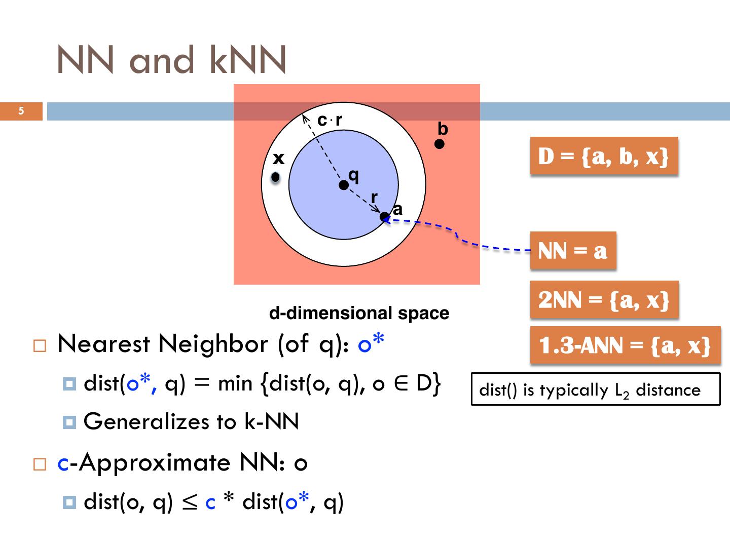
5 . NN and kNN 5 c!r b x D = {a, b, x} q r a NN = a d-dimensional space 2NN = {a, x} ¨ Nearest Neighbor (of q): o* 1.3-ANN = {a, x} ¤ dist(o*, q) = min {dist(o, q), o ∈ D} dist() is typically L2 distance ¤ Generalizes to k-NN ¨ c-Approximate NN: o ¤ dist(o, q) ≤ c * dist(o*, q) 

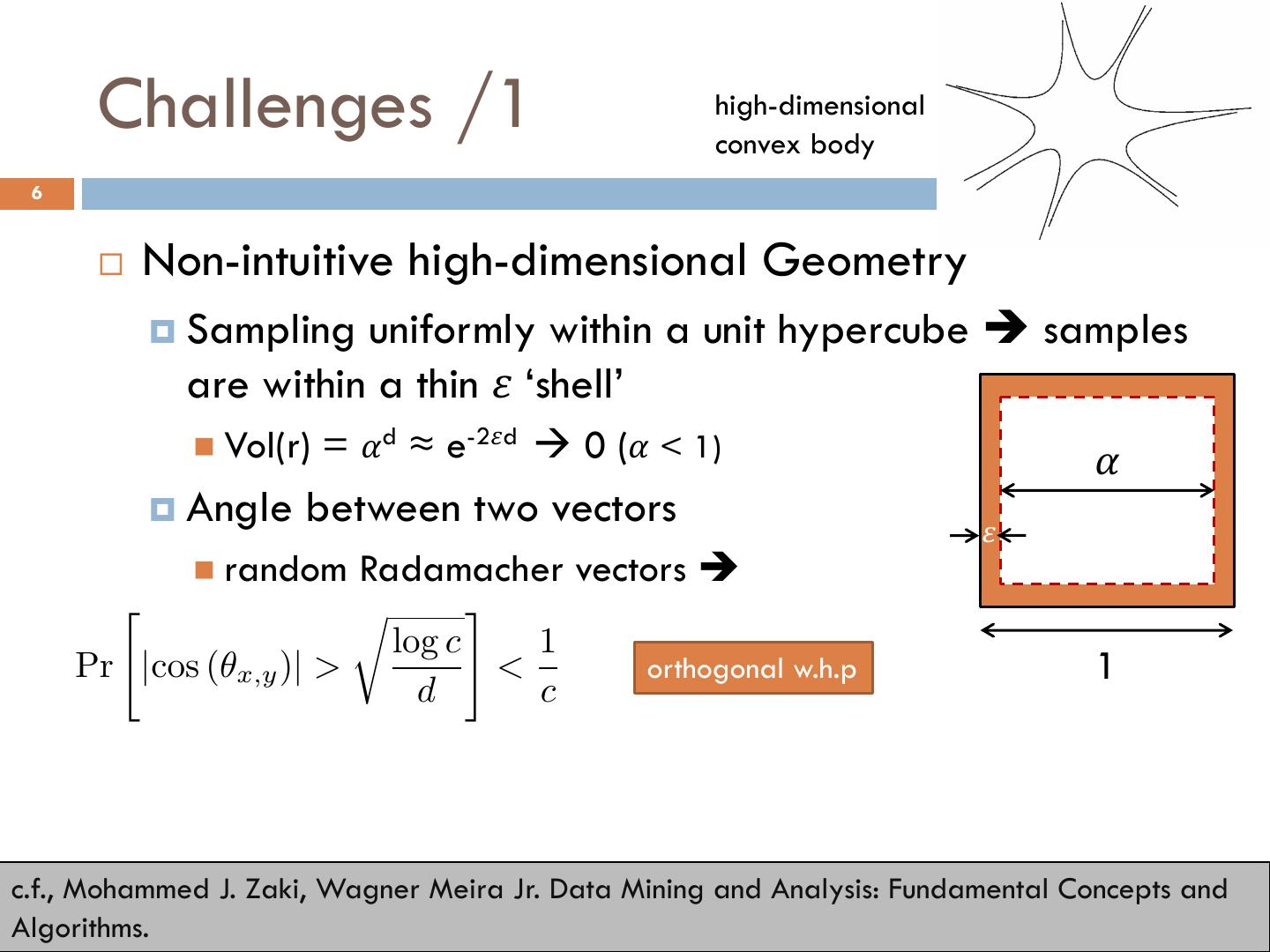
6 . Challenges /1 high-dimensional convex body 6 ¨ Non-intuitive high-dimensional Geometry ¤ Sampling uniformly within a unit hypercube è samples are within a thin 𝜀 ‘shell’ n Vol(r) = 𝛼d ≈ e-2𝜀d à 0 (𝛼 < 1) 𝛼 ¤ Angle between two vectors 𝜀 n random Radamacher vectors è " r # log c 1 Pr |cos (✓x,y )| > < orthogonal w.h.p 1 d c c.f., Mohammed J. Zaki, Wagner Meira Jr. Data Mining and Analysis: Fundamental Concepts and Algorithms. 

7 . Challenges /1 7 ¨ Curse of Dimensionality / Concentration of Measure ¤ Under some assumptions, maxdist(q, D)/mindist(q, D) converges to 1 n Key assumption: independent distribution in each dimension n k-NN is still meaningful for real datasets ¤ Hard to find algorithms sub-linear in n (# of points) and polynomial in d (# of dimensions) ¤ Approximate version (c-ANN) is not much easier c.f., Asymptotic Geometric Analysis, Part I. Shiri Artstein-Avidan, Apostolos Giannopoulos, and Vitali Milman 

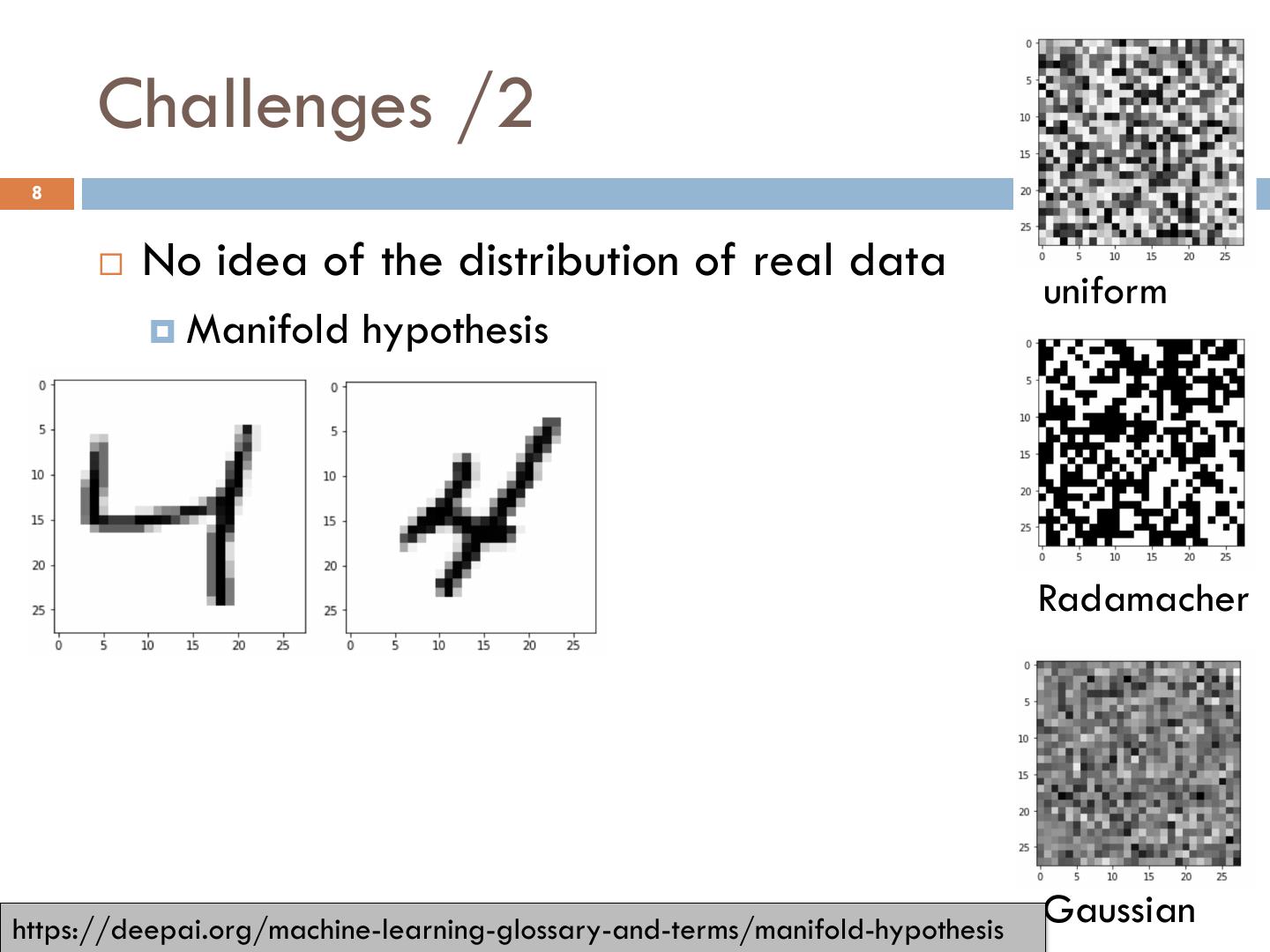
8 . Challenges /2 8 ¨ No idea of the distribution of real data uniform ¤ Manifold hypothesis Radamacher https://deepai.org/machine-learning-glossary-and-terms/manifold-hypothesis Gaussian 

9 . https://colah.github.io/posts/2014-10-Visualizing-MNIST/ Challenges /2 9 ¨ Distribution of Real Data ¤ Manifold hypothesis 

10 . Challenges /3 10 ¨ Large data size ¤ 1KB for a single point with 256 dims è 1B pts = 1TB n ~100 SIFT vectors per image ¤ High-dimensionality (e.g., documents è millions of dimensions) ¨ Variety of distance/similarity functions ¤ Less of an issue in the DL era 

11 . Understanding & Progress 11 ¨ LSH ¨ PQ ¨ Graph-based 

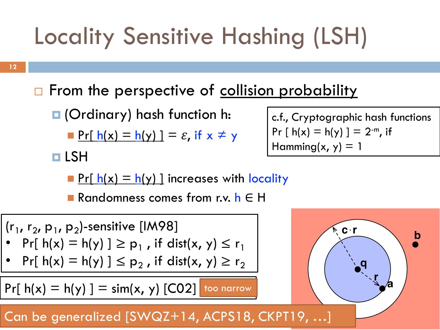
12 . Locality Sensitive Hashing (LSH) 12 ¨ From the perspective of collision probability ¤ (Ordinary) hash function h: c.f., Cryptographic hash functions n Pr[ h(x) = h(y) ] = 𝜀, if x ≠ y Pr [ h(x) = h(y) ] = 2-m, if Hamming(x, y) = 1 ¤ LSH n Pr[ h(x) = h(y) ] increases with locality n Randomness comes from r.v. h ∈ H (r1, r2, p1, p2)-sensitive [IM98] c!r b • Pr[ h(x) = h(y) ] ≥ p1 , if dist(x, y) ≤ r1 • Pr[ h(x) = h(y) ] ≤ p2 , if dist(x, y) ≥ r2 q r a Pr[ h(x) = h(y) ] = sim(x, y) [C02] too narrow Can be generalized [SWQZ+14, ACPS18, CKPT19, …] 

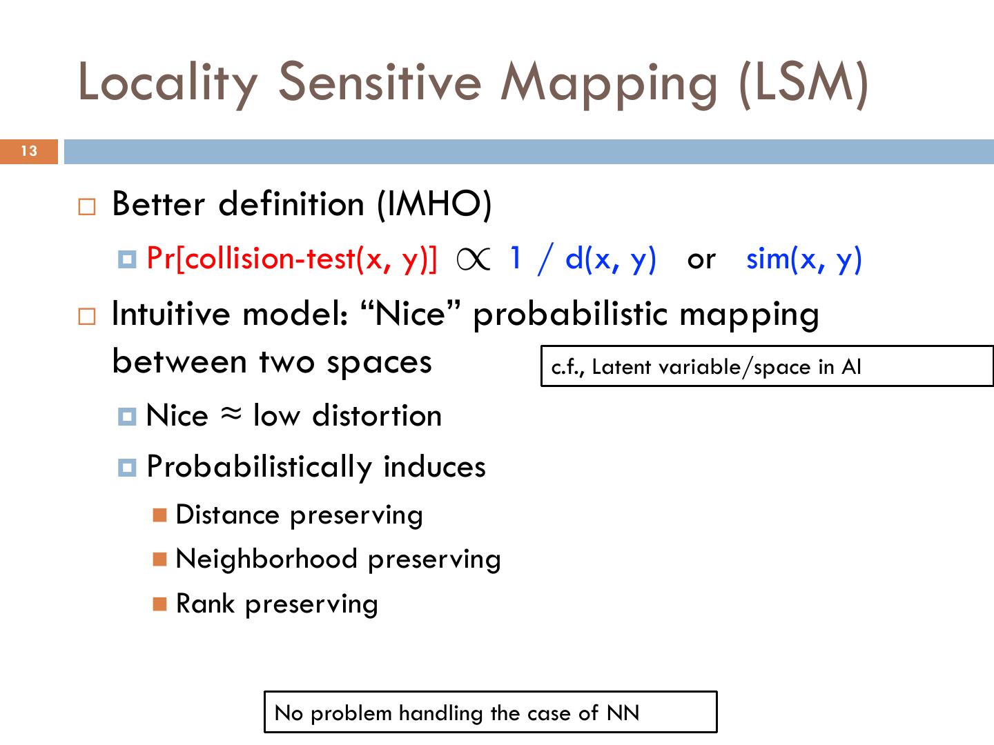
13 . Locality Sensitive Mapping (LSM) 13 ¨ Better definition (IMHO) ¤ Pr[collision-test(x, y)] / 1 / d(x, y) <latexit sha1_base64="bHWpAmhnEaScGFcHWtstDwFeVn8=">AAAB73icbVBNSwMxEJ2tX7V+VT16CRbBU9mVoh6LXjxWsB/QLiWbZtvQbBKTrFCW/gkvHhTx6t/x5r8xbfegrQ8GHu/NMDMvUpwZ6/vfXmFtfWNzq7hd2tnd2z8oHx61jEw1oU0iudSdCBvKmaBNyyynHaUpTiJO29H4dua3n6g2TIoHO1E0TPBQsJgRbJ3U6SktlZWlfrniV/050CoJclKBHI1++as3kCRNqLCEY2O6ga9smGFtGeF0WuqlhipMxnhIu44KnFATZvN7p+jMKQMUS+1KWDRXf09kODFmkkSuM8F2ZJa9mfif101tfB1mTKjUUkEWi+KUIyvR7Hk0YJoSyyeOYKKZuxWREdaYWBfRLIRg+eVV0rqoBpfV2n2tUr/J4yjCCZzCOQRwBXW4gwY0gQCHZ3iFN+/Re/HevY9Fa8HLZ47hD7zPH9zhj90=</latexit> or sim(x, y) ¨ Intuitive model: “Nice” probabilistic mapping between two spaces c.f., Latent variable/space in AI ¤ Nice ≈ low distortion ¤ Probabilistically induces n Distance preserving n Neighborhood preserving n Rank preserving No problem handling the case of NN 

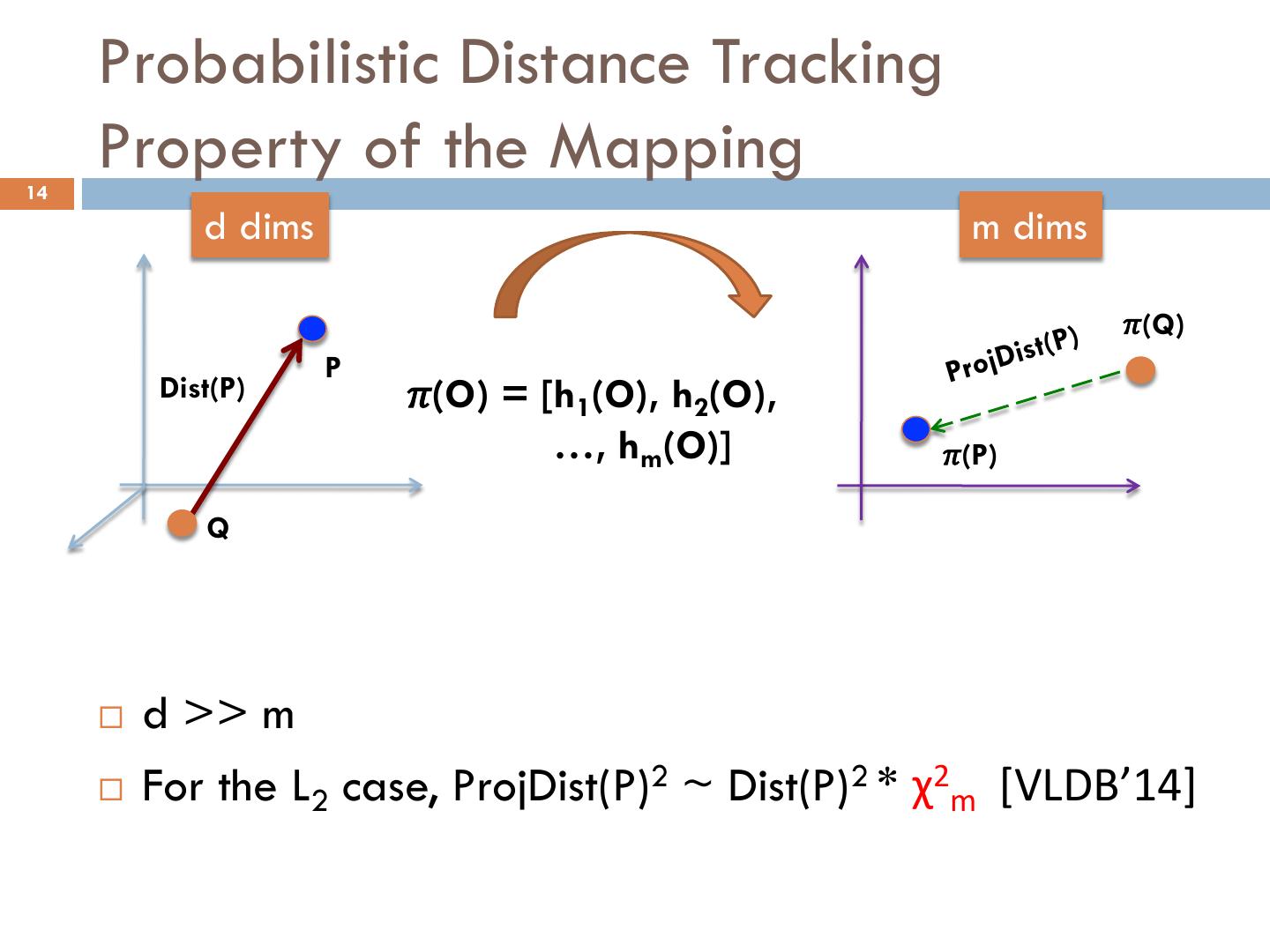
14 . Probabilistic Distance Tracking 14 Property of the Mapping d dims m dims 𝜋(Q) jDist(P) P Pro Dist(P) 𝜋(O) = [h1(O), h2(O), …, hm(O)] 𝜋(P) Q ¨ d >> m ¨ For the L2 case, ProjDist(P)2 ~ Dist(P)2 * χ2m [VLDB’14] 

15 . Making Use of It 15 ¨ “Where can I find the image of my NN point in the projected space?” ¤ Among T-NNs of 𝜋(Q) ¨ T = o(1) * n [VLDB’14] ¨ T = O(c3) ✓ ◆ <latexit sha1_base64="2i+IUG4p0Aheyl1hUgjhI3eXM9E=">AAACG3icbVDLSgNBEJz1bXxFPXoZDIJewm4I6lH04s0IRoVsDLOT3mRwdmaZ6RXCsv/hxV/x4kERT4IH/8bJ4+CroKGo6qa7K0qlsOj7n97U9Mzs3PzCYmlpeWV1rby+cWl1Zjg0uZbaXEfMghQKmihQwnVqgCWRhKvo9mToX92BsUKrCxyk0E5YT4lYcIZO6pRrZ6GEGHfD2DCeB0UeQmqF1OomrxUFDXlXIw2l7lFFQyN6fdzrlCt+1R+B/iXBhFTIBI1O+T3sap4loJBLZm0r8FNs58yg4BKKUphZSBm/ZT1oOapYAradj34r6I5TujTWxpVCOlK/T+QssXaQRK4zYdi3v72h+J/XyjA+bOdCpRmC4uNFcSYpajoMinaFAY5y4AjjRrhbKe8zlxK6OEsuhOD3y3/JZa0a7Ffr5/XK0fEkjgWyRbbJLgnIATkip6RBmoSTe/JInsmL9+A9ea/e27h1ypvMbJIf8D6+AObNoVI=</latexit> 1 𝜋 (o1) ¤ Require m = O ✏2 · log n 𝜋 (o4) 𝜋 (q) 𝜋 (o2) 𝜋 (o3) 

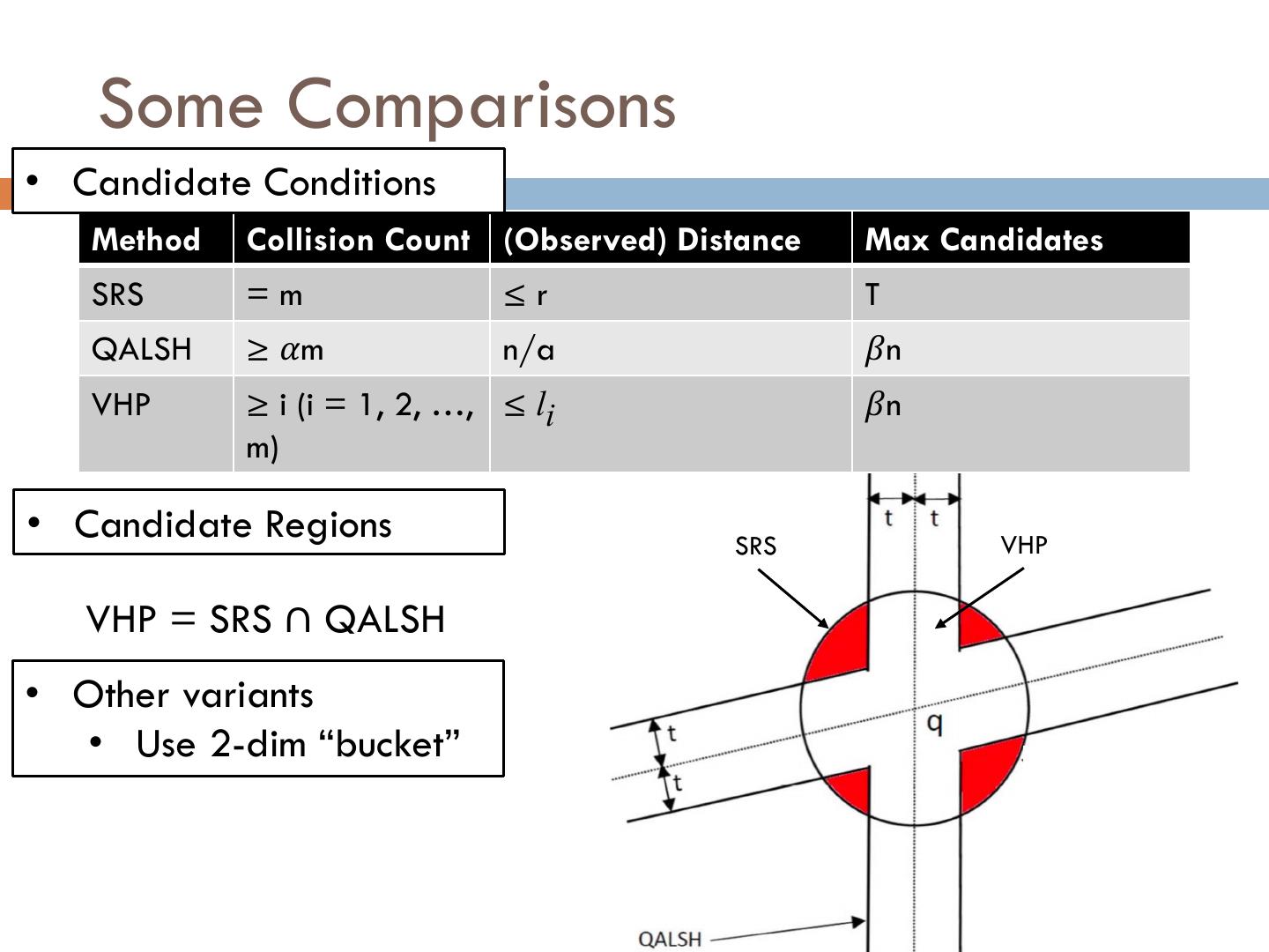
16 . Some Comparisons •16 Candidate Conditions Method Collision Count (Observed) Distance Max Candidates SRS =m ≤r T QALSH ≥ 𝛼m n/a 𝛽n VHP ≥ i (i = 1, 2, …, ≤ li 𝛽n m) • Candidate Regions SRS VHP VHP = SRS ∩ QALSH • Other variants • Use 2-dim “bucket” 

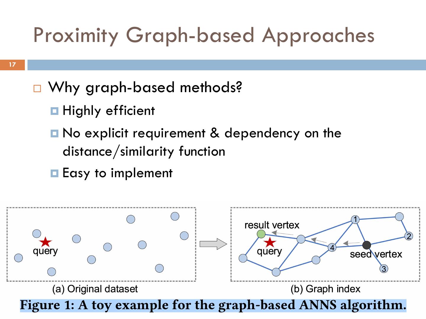
17 . Proximity Graph-based Approaches 17 ¨ Why graph-based methods? ¤ Highly efficient ¤ No explicit requirement & dependency on the distance/similarity function ¤ Easy to implement 

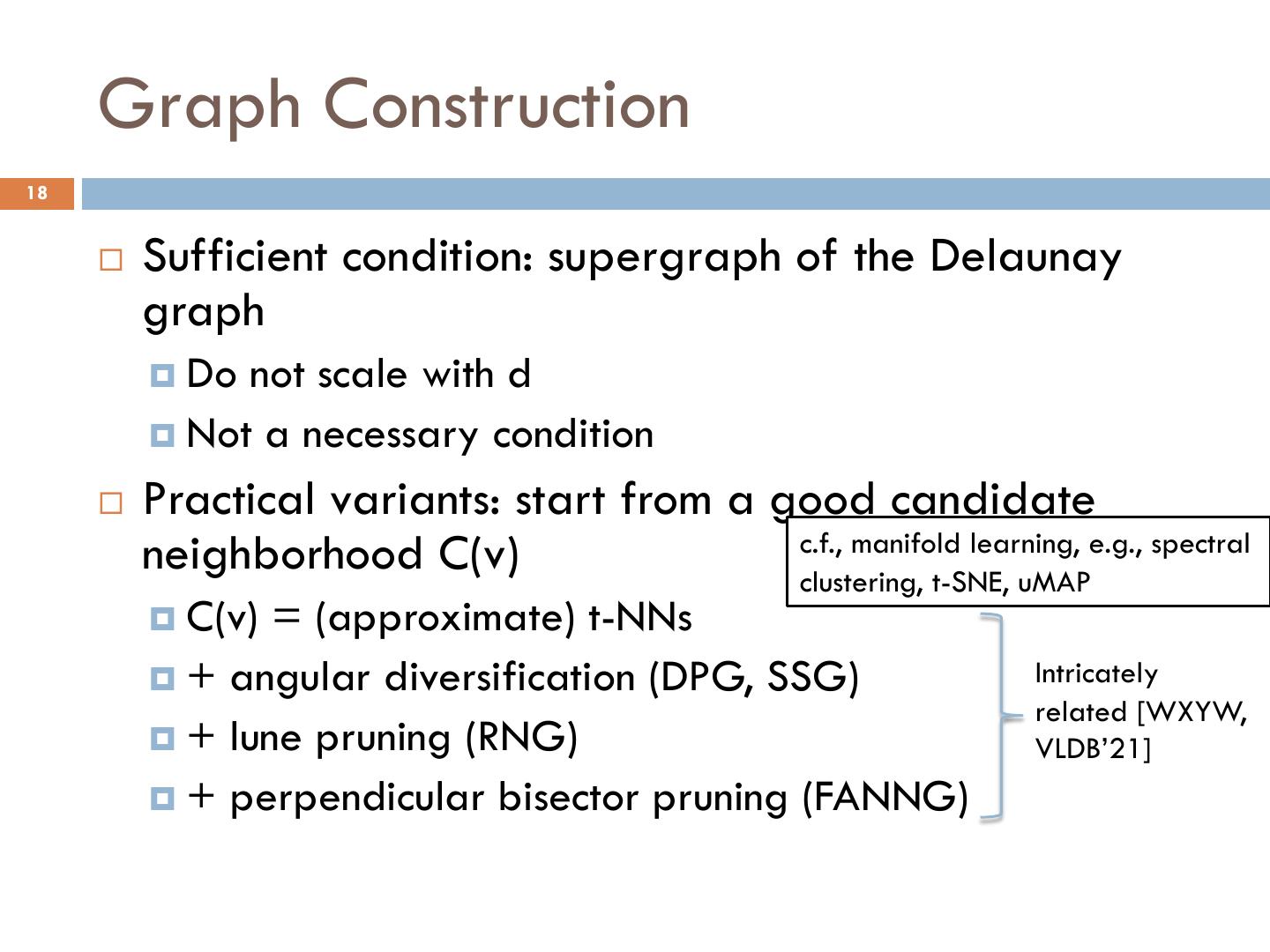
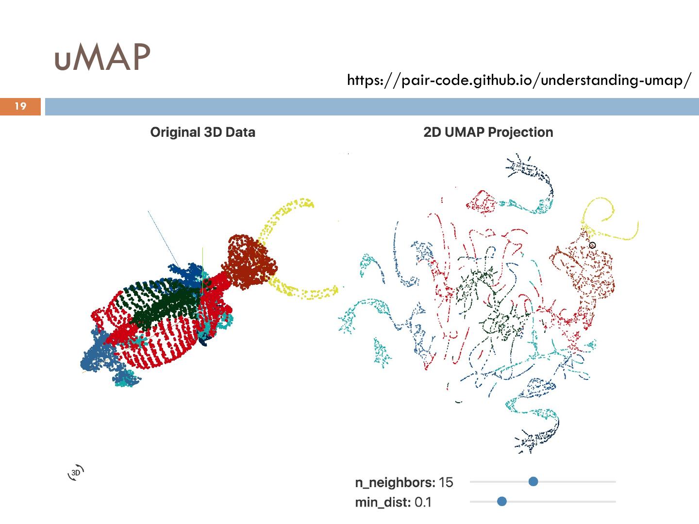
18 . Graph Construction 18 ¨ Sufficient condition: supergraph of the Delaunay graph ¤ Do not scale with d ¤ Not a necessary condition ¨ Practical variants: start from a good candidate neighborhood C(v) c.f., manifold learning, e.g., spectral clustering, t-SNE, uMAP ¤ C(v) = (approximate) t-NNs ¤ + angular diversification (DPG, SSG) Intricately related [WXYW, ¤ + lune pruning (RNG) VLDB’21] ¤ + perpendicular bisector pruning (FANNG) 

19 . uMAP https://pair-code.github.io/understanding-umap/ 19 

20 . Why It Works? 20 ¨ Approach the NN(q) ¨ Dimension 1: ¤ Deterministically: monotonic search path ¤ Probabilistically (under assumptions, e.g., constant doubling dimensionality [STOC’02]; uniform distribution on Sd-1 [SoCG’18]) ¨ Dimension 2: ¤ Greedy search + meta-heuristics (tabu; beam) ¤ Single vs multiple searches ¨ Dimension 3: stage-view ¤ Closing-in + Traversing SCC [arXiv’21] 

21 . Why It Works So Well? 21 ¨ Huge discrepencies between theory and practice ¨ Observations (some examples) ¤ Long-distance edges n [SoCG’18] / HNSW vs empirical results ¤ Clustering coefficient / SCCs 102627 34634 [arXiv’20] vs empirical results 368268 n 128689 286218 20990 83948 141366 268984 77729 139537 top-4 top-6 top-10 153901 103208 120499 76736 top-10 303103 30982 113179 top-3 top-9 top-1 top-4 top-7 166381 top-8 top-1 top-5 7637 256357 21174 242170 top-2 top-7 246234 34543 301581 top-6 top-3 top-5 top-9 top-8 Q40, Audio top-2 Q22, Youtube 

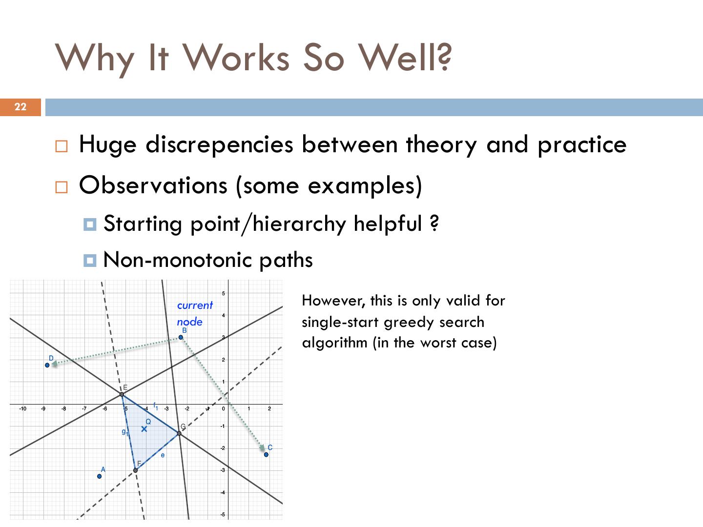
22 . Why It Works So Well? j g 14 22 13 ¨ Huge discrepencies between theory and practice 12 11 ¨ Observations (some examples) 10 9 ¤ Starting point/hierarchy helpful ? 8 ¤ Non-monotonic paths 7 6 However, this is only valid for 5 current single-start greedy search 4 node B 3 algorithm (in the worst case) D 2 1 E -11 -10 -9 -8 -7 -6 -5 -4 f1 -3 -2 -1 0 1 2 3 4 5 6 7 8 9 10 11 12 13 14 15 16 17 18 19 20 21 22 23 Q G -1 g1 -2 C e F A -3 -4 -5 

23 . Recent Progresses: AI for ANN 23 ¨ Learning for index construction ¤ Learning the hash/mapping function (DSH, ICDE’21) ¤ Learning to partition the data [ICLR’21] ¨ Learning for query processing ¤ Learning to route [ICML’19] ¤ Learning to terminate [SIGMOD’21, arXiv’21] ¤ Learning to access data [arXiv’20] ¨ Miscellaneous ¤ Learning a space transformation [ICLR’19] ¤ Learning to compute distance [TPAMI’21] 

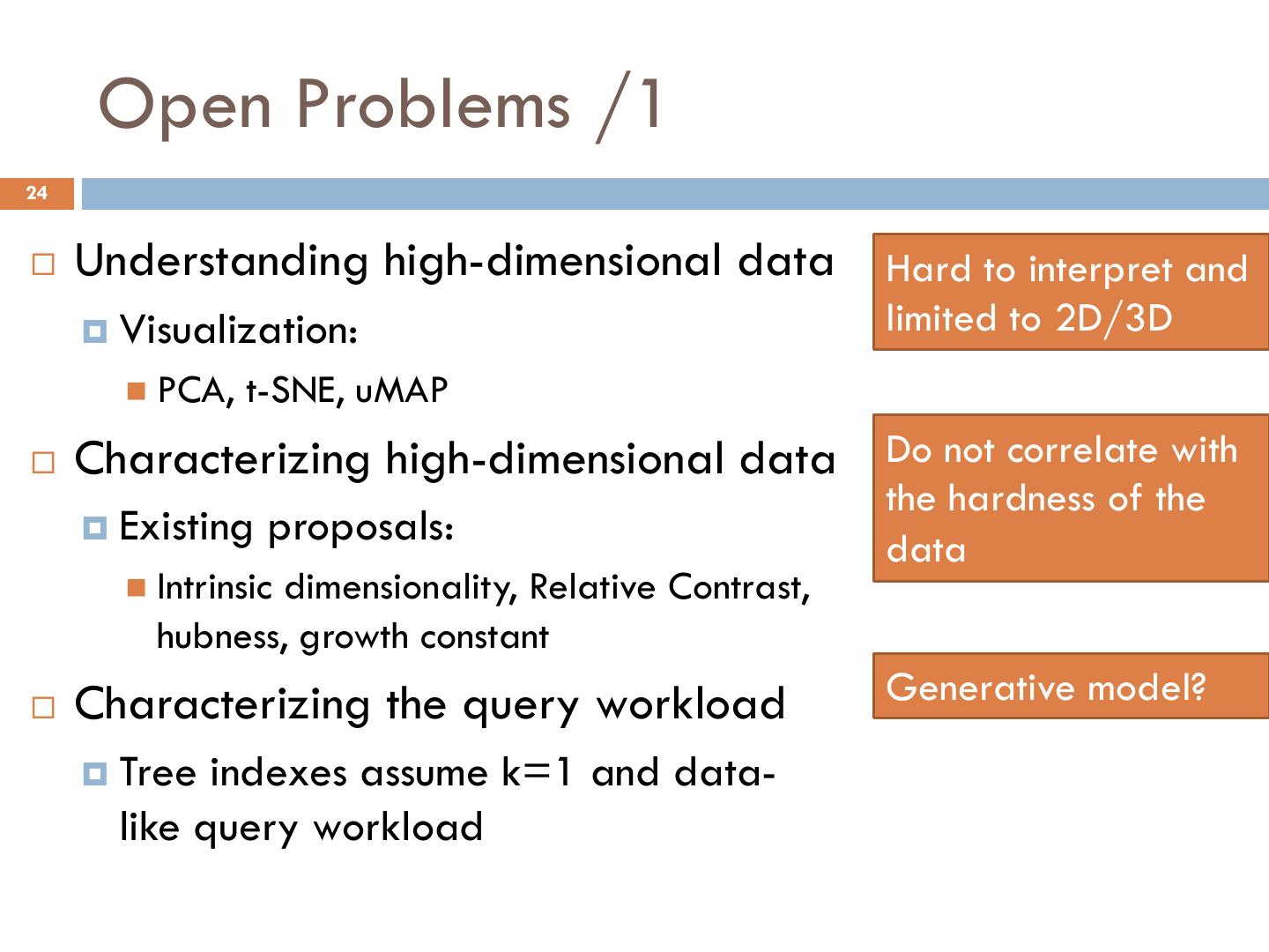
24 . Open Problems /1 24 ¨ Understanding high-dimensional data Hard to interpret and ¤ Visualization: limited to 2D/3D n PCA, t-SNE, uMAP ¨ Characterizing high-dimensional data Do not correlate with the hardness of the ¤ Existing proposals: data n Intrinsic dimensionality, Relative Contrast, hubness, growth constant ¨ Characterizing the query workload Generative model? ¤ Tree indexes assume k=1 and data- like query workload 

25 . Open Problems /2 25 ¨ Understand which properties are important for Proximity Graph-based approach ¨ Proximity graph index & search algorithm ¤ Chicken-and-egg problem? Joint optimization? ¤ Is monotonic path/greedy search important? ¨ Scalability issue ¨ AI can help? 

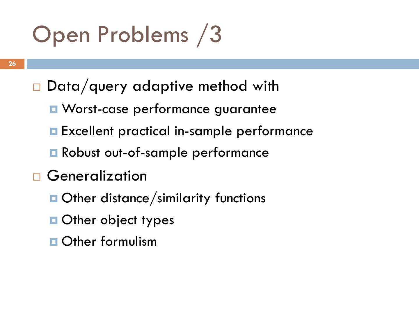
26 . Open Problems /3 26 ¨ Data/query adaptive method with ¤ Worst-case performance guarantee ¤ Excellent practical in-sample performance ¤ Robust out-of-sample performance ¨ Generalization ¤ Other distance/similarity functions ¤ Other object types ¤ Other formulism 

27 . Open Problems /4 27 ¨ Evaluation ¤ Comprehensive n Algorithms n Datasets n Random hypercube/sphere n Sparse / intermediate / dense regions (d vs log(n)) n Distribution / local/instrinsic dimensionality n Result distribution ¤ Fair ¤ Forward-looking ¨ Systems ¤ Integration (esp. with DB & AI pipelines) ¤ More capabilities (e.g., mixing with other predicates) 

28 . Q&A 28 Thank You ! Wei Wang weiwcs@ust.hk http://www.cse.ust.hk/~weiwcs